|
This is an overview of the Benchmarking Sorting Algorithms project I completed for the Computational Thinking with Algorithms module at GMIT as part of the Higher Diploma in Data Analytics.
The project specification was as follows:
- Write a Python application to benchmark five different sorting algorithms.
- Write a report which introduces the algorithms you have chosen and discusses the results of the benchmarking process.
The five sorting algorithms which you will implement, benchmark and discuss in this project must be chosen according to the following criteria:
- A simple comparison-based sort (Bubble Sort, Selection Sort or Insertion Sort)
- An efficient comparison-based sort (Merge Sort, Quicksort or Heap Sort)
- A non-comparison sort (Counting Sort, Bucket Sort or Radix Sort)
- Any other sorting algorithm of your choice
- Any other sorting algorithm of your choice
The project which was submitted on the college Moodle platform included a final report in pdf format together with the .py Python source code files in a single zip file.
Here is an HTML version of the complete report for the project, of which some extracts are included below.
In the introduction section I introduce the concept of sorting algorithms, discussing the relevance of concepts such as time and space complexity, performance, in-place sorting, stable sorting, comparator functions, comparison-based and non-comparison-based sorts.
The section on sorting algorithms provides an overview of five sorting algorithms and looks at their time and space complexities. The five sorting algorithms introduced here are as follows:
- Bubble Sort as an example of a simple comparison-based sorting algorithm.
- Merge Sort as an example of an efficient comparison-based sorting algorithm.
- Counting Sort as an example of a non-comparison based sorting algorithm.
- Insertion Sort - another simple comparison-based sorting algorithm.
- Quick Sort - another efficient comparison-based sorting algorithm.
The report includes for each sorting algorithm
- a description of how each sorting algorithm works
- a discussion of each sorting algorithm’s time and space complexity
- a diagram illustrating how each of the sorting algorithms works on a small input array
- Python code for implementing each sorting algorithm and an analysis of each algorithm’s performance.
The code for sorting algorithms is widely available online and in books and all sources referred to are acknowledged. For each of the 5 sorting algorithms a diagram illustrates the
Implementation and Benchmarking
In the implementation and benchmarking section of the report I describe the process I followed when implementing my benchmarking application, describing in detail how the application code works. The python code for the application is also included in this section of the report.
The purpose of the benchmarking application is to take arrays of randomly generated integers of varying input sizes and to test the effect of the input size on the running time of each sorting algorithm. The running time for each algorithm is measured 10 times and the averages of the ten runs for each sorting algorithm and for each input size is then output to the console when the program has finished executing. The application also generates a plot of the resulting averages. The elapsed times for each individual run for each type of algorithm of each input array size are exported to csv file for reference. The average times are also exported to another csv file.
Python’s random module was used to create random array sizes that varied from 100 integers to 10,000 integers. The time function from the time module function records time in seconds from the epoch.
The program consists of an outer for loop which iteratates through each of the different sorting algorithms provided to it, a nested for loop which iterates through each of the sizes in the size arrays and another nested for loop which iterates the number of times provided to the runs parameter. Within the inner for loop, a new random array is created each time using the size as the number of random elements. Each sorting function is called 10 times for each different size array. A new random array is created each time.
The time is taken immediately before the sorting function sorts the data and immediately after the sorting function sorts the data. The elapsed time is calculated as the difference between the two times. The creation of the random array itself is not timed.
At each run, the elapsed time, the run number (1 to 10), the name of the sorting function and the size of the input array sorted each time is recorded in lists. The results of each trial for each type of sorting algorithm for each input size to be sorted is then output to a pandas DataFrame. This contains the results of each individual trial in seconds. Another function is then called by the main program which takes the DataFrame containing the raw elapsed times and calculates the averages to 3 decimal places of the 10 different runs for each sort algorithm for each input size. The pandas groupby function is used here to get the averages grouped by the sorting function name and the input array size. The results are multiplied by 1000 to get the averages in milliseconds. The results of the groupby operation is then unstacked to get the results in the desired format for this benchmarking project. The main function also calls another function to plot the averages using the matplotlib.pyplot module and the seaborn library resulting in a graph showing the average times in milliseconds on the vertical axis and the size of the input array on the horizontal axis.
When testing the program, print statements were used to ensure that the resulting dataframe of elapsed times did indeed contain the correct elapsed time for each trial for each algorithm at each input size. The dictionary of sorting algorithms could be changed to test the performance of a single sorting algorithm or a combination of algorithms.
A copy of the benchmarking.py script is included in the project report in the Python Benchmarking application code section.
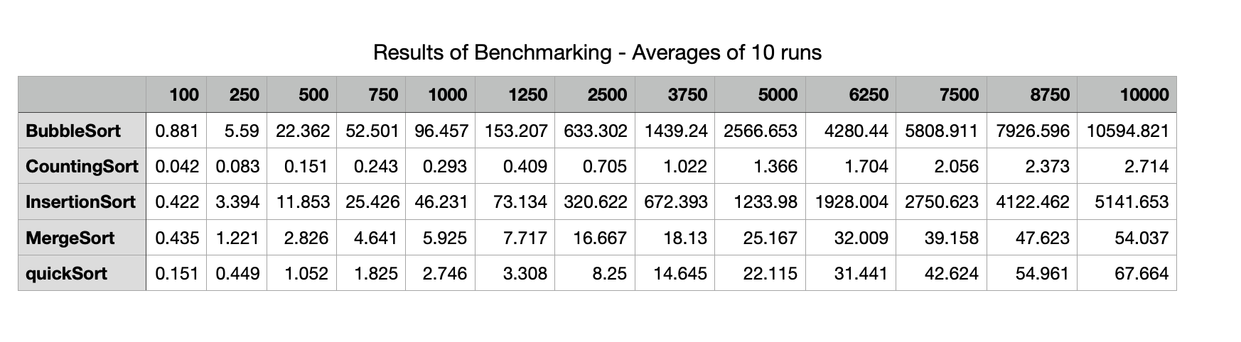
The results of the benchmarking of the 5 sorting algorithms are then presented through the use of a table that compares each sorting algorithm and a graph of the average times recorded for each of the sorting algorithms.
The table below shows the average times in milliseconds across the 10 runs for each sorting algorithm using the different sized inputs from 100 elements up to 10,000 elements. The table shows that Bubble Sort takes over 10 seconds to sort a random array containing 10,000 random integers while Counting Sort performs the same task in less than 3 milliseconds. Insertion Sort here takes about half the time as Bubble Sort. Merge Sort and Quick Sort and Merge Sort have times of the same order. The plots illustrate the performance of the five sorting algorithms and how they differ from each other.
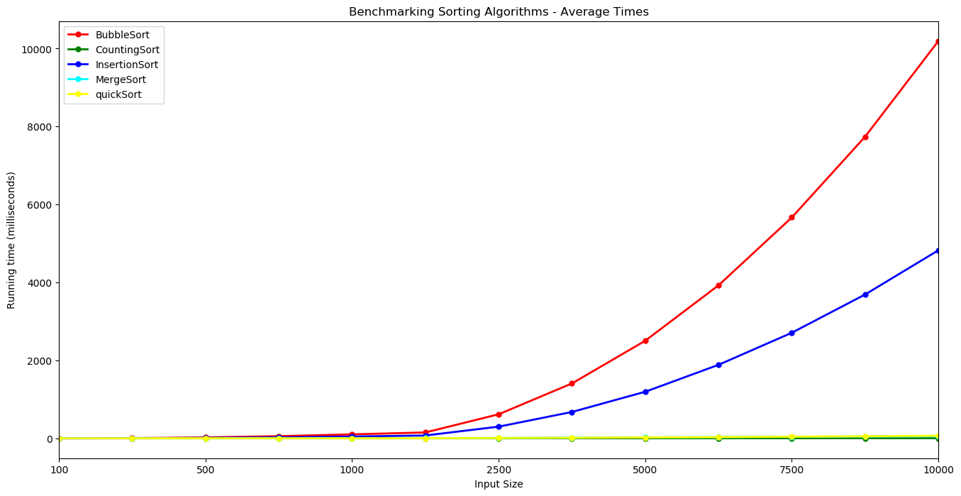
Bubble Sort increases at a faster rate, followed by Insertion Sort. These algorithms display an $n^2$ growth rate. It is hard to distinguish Counting Sort, Merge Sort and Quick Sort here given the scale of the y-axis which is dominated by the very slow times for Bubble Sort.
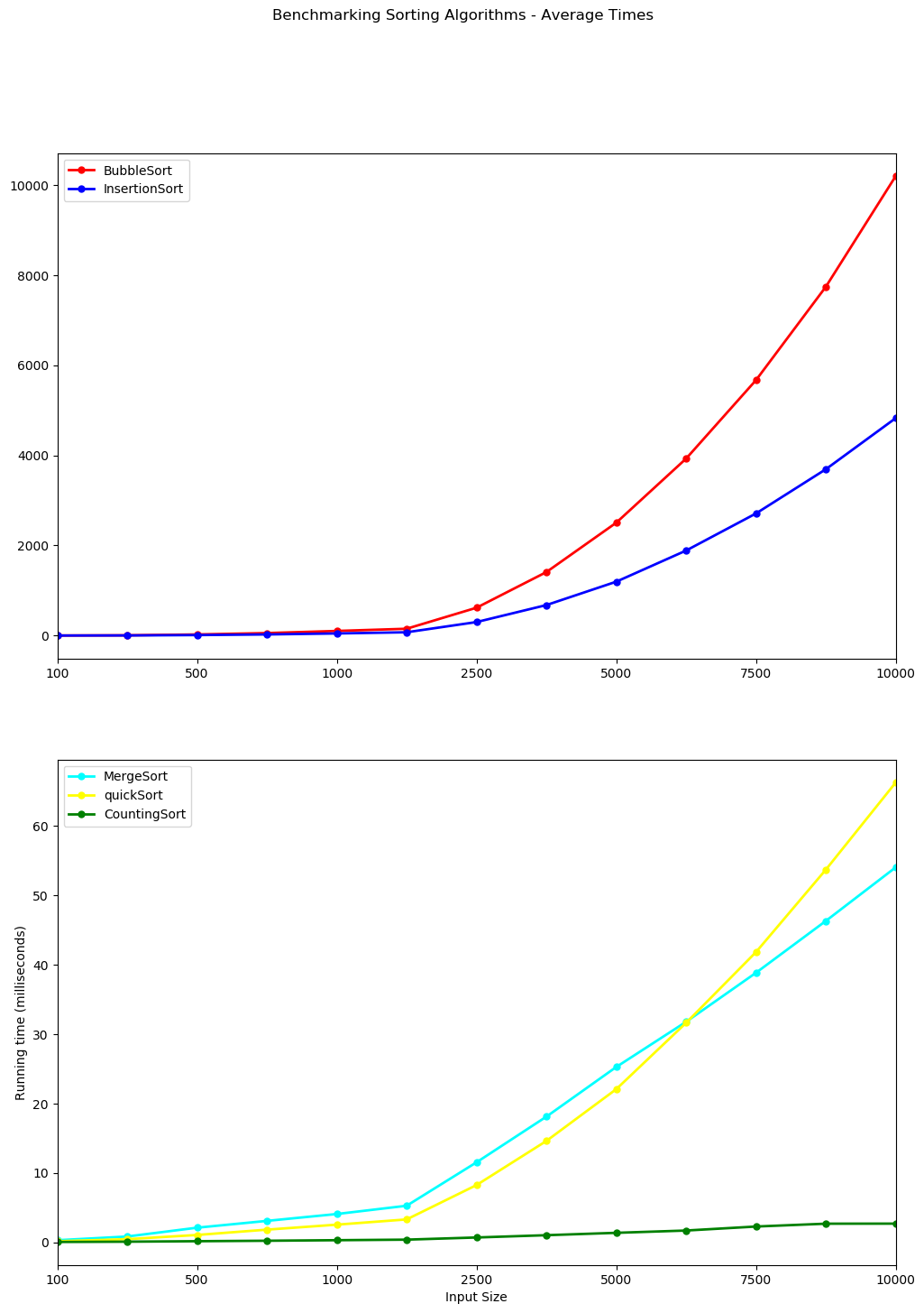
Bubble Sort and Insertion Sort are therefore plotted together below on a single plot while Counting Sort, Merge Sort and Quick Sort are plotted on a separate graph. Note the y-axis are on different scales. The y-axis for Bubble Sort and Insertion sort climbs to 10,000 milliseconds or ten seconds while the scale for the other 3 is less than 70 milliseconds.
The 5 sorting algorithms used in this benchmarking project
1. Simple comparison-based sorts
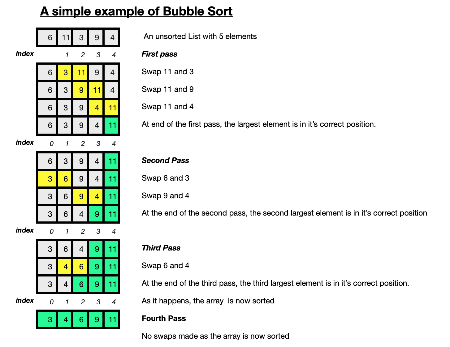
Bubble Sort is a fairly simple comparison-based sorting algorithm and is so named for the way larger values in a list “bubble up” to the end as sorting takes place. The algorithm repeatedly goes through the list to be sorted, comparing and swapping adjacent elements that are out of order. With every new pass through the data, the next largest element bubbles up towards it’s correct position. Although it is quite simple to understand and to implement, it is slow and impractical for most problems apart from situations where the data is already nearly sorted.
Bubble Sort works by repeatedly comparing neighbouring elements and swapping them if they are out of order. Multiple passes or iterations are made through the list and with each pass through the list, the next largest element ends up in it’s proper place.
The diagram below is a simple example of Bubble sort on a small unsorted list containing 5 elements.
The section on analysing Bubble Sort looks at the performance of the bubble sort algorithm. The worst case scenario for Bubble sort occurs when the data to be sorted is in reverse order. The average case is when the elements of the array are in random order.
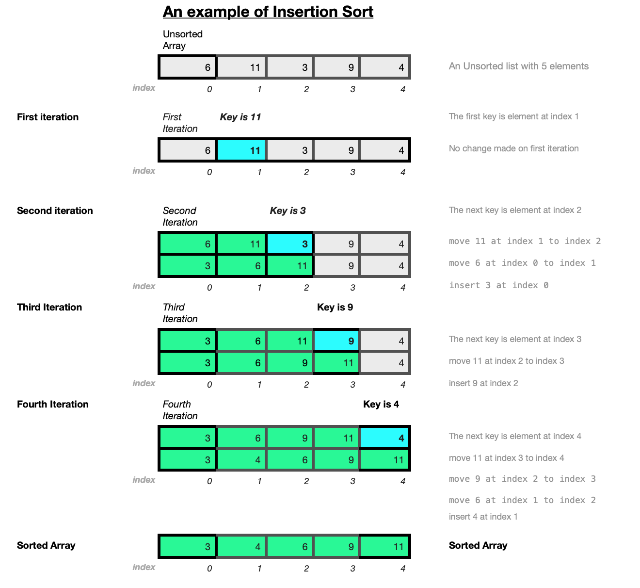
Insertion sort is a simple sorting algorithm that builds the final sorted array (or list) one item at a time. It is much less efficient on large lists than more advanced algorithms such as quicksort, heapsort, or merge sort.
The Insertion Sort algorithm is relatively easy to implement and understand as it can be compared to sorting a deck of cards. The first element is assumed to be sorted. The sorted list is built one element at a time by comparing each item with the rest of the items in the list, then inserting the element into its correct position. After each iteration, an unsorted element has been placed in it’s right place.
Insertion Sort is an iterative algorithm. The diagram below illustrates how the Insertion Sort algorithm works on a small array of random integers a=[6,11,3,9,4].
The section on analysing Insertion Sort looks at it’s performance. The best case would occur on a list that is already sorted. The inner loop does not need to iterate at all on a list that is already sorted. Insertion sort is the only comparison-based sorting algorithm that does this. The inner loop only iterates until it finds the insertion point.
The Insertion Sort differs from other simple sorting algorithms such as Bubble Sort and Selection Sort in that while values are shifted up one position in the list, there is no exchange as such. Insertion Sort is a stable in-place sorting algorithm. It works well on small lists and lists that are close to being sorted but is not very efficient on large random lists. It’s efficiency increased when duplicate items are present.
Efficient comparison based sorts
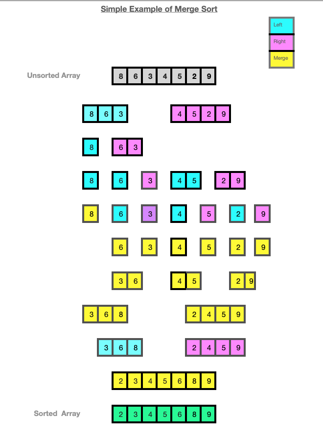
Merge Sort is an efficient, general-purpose, comparison-based sorting algorithm. This divide-and-conquer algorithm was proposed by John von Neumann in 1945 and uses recursion to continually split the list in half. A divide-and-conquer algorithm recursively breaks a problem down into two or more sub-problems of the same or related type until these become simple enough to be solved directly. Then the solutions to the sub-problems are combined to produce a solution to the original problem.
The list is divided into two evenly (as much as possible) sized halves which is repeated until the sublist contains a single element or less. Each sub-problem is then sorted recursively and the solutions to all the sub-lists are combined or merged into a single sorted new list. A list with one or less elements is considered sorted and is the base case for the recursion to stop. This algorithm will need extra memory to copy the elements when sorting. The extra space stores the two halves extracted using slicing.
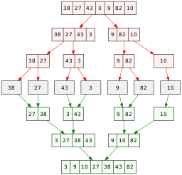
The diagram below demostrates how the MergeSort algorithm works on a small array of random integers [8, 6, 3, 4, 5, 2, 9].
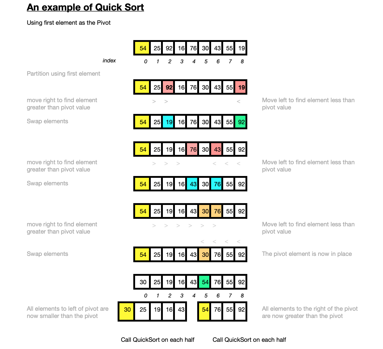
The Quick Sort algorithm is somewhat similar to Merge Sort as it a comparison-based algorithm that uses a recursive divide-and-conquer technique. It does not however need the extra memory that Merge Sort requires. A pivot element is used to divide the list for the recursive calls to the algorithm.
The QuickSort algorithm is also known as the partition-exchange sort and when implemented well, it can be about two or three times faster than its main competitors, merge sort and heapsort.
The key part of the quick sort algorithm is the partitioning which aims to take an array, use an element from the array as the pivot, place the pivot element in its correct position in the sorted array, place all elements that are smaller than the pivot before the pivot and all the elements that are larger than the pivot after the pivot element.
A pivot element is chosen, elements smaller than the pivot are moved to the left while elements greater than the pivot are moved to the right. The array elements are reordered so that any array elements less than the pivot are placed before the partition while array elements with values greater than the pivot element come after. After the partioning, the pivot will be in it’s final position.
The diagram here shows how the Quick Sort algorithm works on a small array of random integers [54,25,92,16,76,30,43,55,20].
The worst-case scenario for Quick Sort depends on the chosen pivot point. The worst case occurs when the array to be sorted is already sorted in the same order or in reverse order or if all elements are the same. If a random element or a median element is instead chosen for the pivot the worst cases are unlikely to occur unless the maximum or minimum element happens to always be selected as the pivot. In practice it is one of the fastest known sorting algorithms, on average.
Non-comparison based sorts
The Counting sort algorithm which was proposed by Harold H. Seward in 1954, is an algorithm for sorting a collection of objects according to keys that are small integers. It is an integer sorting algorithm that counts the number of objects that have each distinct key value, and using arithmetic on those counts to determine the positions of each key value in the output sequence.
While comparison sorts such as Bubble Sort and Merge Sort make no assumptions about the data, comparing all elements against each other, non-comparison sorts such as Counting Sort do make assumptions about the data, such as the range of values the data falls into and the distribution of the data. In this way the need to compare all elements against each other is avoided. Counting Sort allows for a collection of items to be sorted in close to linear time which is made possible by making assumptions about the type of data to be sorted.
The Counting Sort algorithm uses keys between a specific range and counts the number of objects having distinct key values. To implement it you first need to determine the maximum value in the range of values to be sorted which is then used to define the keys. The keys are all the possible values that the data to be sorted can take. An auxillary array is created to store the count of the number of times each key value occurs in the input data.
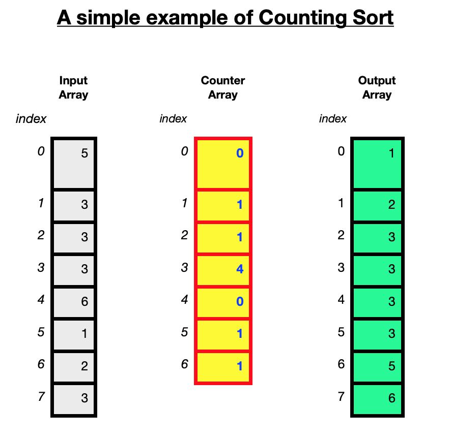
The Counting Sort algorithm sorts the elements of a list by counting the number of occurences for each unique element in the list. This count is stored in another counter array. The sorting is performed by mapping the count as an index of the counter array. Go through the array of input data and record how many times each distinct key value occurs. The sorted data in then built based on the frequencues of the key values stored in this count array.
The diagram below illustates how the counting sort algorithm works using an unsorted array of 8 integers [5, 3, 3, 3, 6, 1, 2, 3]. The maximum value in the array is 6.
The best, worst and average complexities for counting sort will always be the same because it doesn’t matter what order the elements are in the array to be sorted, the algorithm will still have to iterate $n+l$ times where $n$ is the size of the array to be sorted and $k$ is the largest value in the array which determines the size of the counter array
The space complexity depends on the maximum value in the data to be sorted. A larger range of elements requires a larger counter array.
Counting Sort is considered suitable for use only with smaller integers which have multiple counts. This is demonstrated in the example above.
Summary and conclusions
The benchmarking in this project looked specifically at the time complexity of the 5 mentioned sorting algorithms. The times were measured and compared to each other and to the expected results given in the studies. The actual times depended on various factors specific to the machine on which they were implemented and therefore the numbers will not match the results other studies might report, given the differences on which they are run. The tests here were run over ten times and the averages taken. The random arrays generated for each run contained random integers between 0 and 100. Using a wider range of integers may affect the performance of each algorithm. While the results in this benchmarking project showed the Counting Sort algorithm as being the fastest, it should be noted that the performance of the Counting Sort algorithm does decrease when the values to be sorted are large. As well as the size of the input, the characteristics of the data may also have an effect on the running time. For this benchmarking project, although different random arrays were used for each run, the characteristics of the data remained the same and the average results used. The average case defines the expected behaviour when executing the algorithm on random input instances. When the averages of all five sorting algorithms are plotted, it is clear than Counting Sort is a far faster sorting algorithm than the two simple sorting algorithms Bubble Sort and Insertion Sort. Insertion sort outperforms Bubble Sort in terms of speed but they are still of the same order of magnitude with a growth rate of $n^2$ . This is expected average case complexity which occurs when the data provided is in random order as it was here. Insertion Sort is not very efficient on large random datasets. Merge Sort and Quick Sort have similar linearithmic growth rates. The results of the benchmarking here are in line with the results expected given the details as outlined earlier for each of the five sorting algorithms studied and summarised in the table below.
Summary of time and space complexities of the five sorting algorithms
| Algorithm | Best Case | Worst Case | Average Case | Space Complexity |
|---|---|---|---|---|
| Bubble Sort | $n$ | $n^2$ | $n^2$ | 1 |
| Insertion Sort | $ n$ | $n^2$ | $n^2$ | 1 |
| Merge Sort | $n log n$ | $n log n$ | $n log n$ | $O(n)$ |
| Quick Sort | $n log n$ | $n^2$ | $n log n$ | $n$ |
| Counting Sort | $(n + k)$ | $(n + k)$ | $(n + k)$ | $(n + k)$ |