The first task was a write a Python function that calculates and prints the square root of two to 100 decimal places in plain Python without using any module from the Python standard library or otherwise. This sounds easier than it was! Like pi the square root of two is an irrational number. An irrational number has an infinite number of decimal points with no recurring pattern.
This task looked at the following:
Various methods for calculating the square root of a number including the The Babylonian Method and Newton’s Method
How irrational numbers are stored on computers
The issues and limitations related to floating-point arithmetic in Python and other programming languages, in particular the problems with accuracy to high levels of precision. Also the problems that may arise when converting from one format to another.
Task 2: The Chi-square ($\chi^2$) Test for independence
$$\chi^2=\sum_{i=1}^{k}\frac{(O_i-E_i)^2}{E_i}$$
The second task involved verifying the Chi-squared test statistic as reported in this Wikipedia article and calculating the p-value.
Wikipedia contributors, “Chi-squared test — Wikipedia, the free encyclopedia,” 2020, [Online; accessed 1-November-2020]. [Online]. Available: https://en.wikipedia.org/w/index.php?title=Chi-squared test&oldid=983024096
Collar
A
B
C
D
Total
White Collar
90
60
104
95
349
Blue Collar
30
50
51
20
151
No Collar
30
40
45
35
150
Total
150
150
200
150
650
The Chi-squared test for independence is a statistical hypothesis test. It is used to analyse whether two categorical variables are independent, to determine if there is a statistically significant difference between the expected frequencies and the observed frequencies in one or more categories of a contingency table.
This task involved the following:
Explaining how the Chi-squared test of independence of a pair of random variables works.
Calculating the Chi-squared statistic using Panda DataFrames to illustrate.
Using the Scipy.Stats module to calculate the Chi-sqaured statistic and associated p-values.
Interpreting the results of the Chi-squared tests.
Task 3: Compare the STDDEV.P and STDDEV.S excel functions
Use NumPy to perform a simulation demonstrating that the STDDEV.S calculation is a better estimate for the standard deviation of a population when performed on a sample.
This task involved the following:
A comparison of the population variance and the sample variances.
The population variance is calculated using the formula:
$$\sigma^2\frac{=\sum(x_i-\mu)^2}{n}$$
The sample variance is calculated using the formula:
$$S^2\frac{=\sum(x_i-\bar{x})^2}{n-1}$$
$n-1$ is usually used in the sample variance formula instead of n because using n tends to produce an underestimate of the population variance.
According to wikipedia, using $n-1$ instead of $n$ in the formula for the sample variance and sample standard deviation is known as Bessel’s Correction, named after Friedrick Bessel.
I simulated data using Numpy.random’s standard_normal function
10,000 data points were put into 1,000 sub-arrays of size 10 to represent 1,000 samples each containing 10 observations each.
The mean of each sample was calculated using Numpy’s mean() function.
The variances and standard deviations are calculated using Numpy’s var and std() functions.
The unbiased variances and standard deviations were calculated using Numpy’s var() and std() functions with the ddof parameter set to $n-1$ instead of the default $n$.
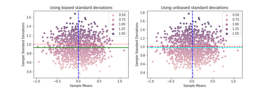
The sample means and variances from each sample were then plotted and compared to the population parameters.
The plots above show that the means are clusted around the population mean of zero which is shown by the vertical blue dashed line. Some sample means are below and some are above and some more are quite a bit away from the population mean. This would depend on the actual values in each sample. Similarly with the standard deviations. The dashed red horizontal line represents the population standard deviation of 1. Again while the sample sample standard are clustered around them, some sample standard deviations are above, some below and some more extreme than others. However when the mean of the sample standard deviations are plotted you can see that the mean of the unbiased standard deviations are closer to the actual standard devision of the population than the mean of the biased sample standard deviations.
Comparing Biased Vs Unbiased standard deviations
I also looked at the means of the sample standard deviations for various small sample sizes between 2 and 6. With a smaller sample size you are more likely to get a sample mean that is a bad estimate for the population mean and you are more likely to significantly underestimate the sample variance.
The plots can be seen in the here in the project notebook.
If a sample is taken from this population, the sample mean of this sample could be very close to the population mean or it might not be depending on which data points are actually in the sample and if the sample points came from one end or other of the underlying population. The mean of the sample will always fall inside the sample but the true population mean could be outside of it. For this reason you are more likely to be underestimating the true variance. The standard deviation is the square root of the variance. Dividing by $n-1$ as shown above instead of $n$ will give a slightly larger sample variance which will be an unbiased estimate.
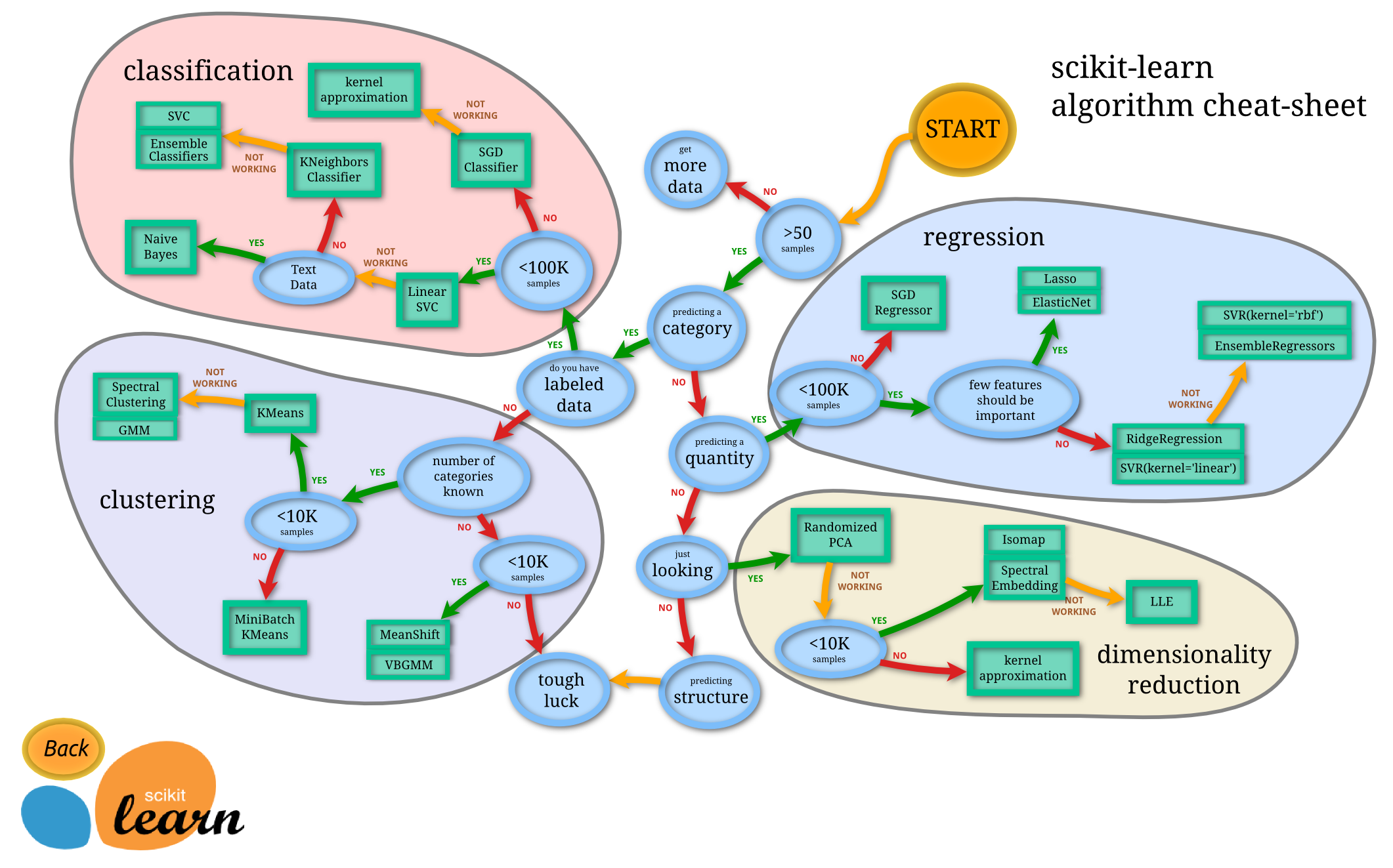
Task 4: Use Scikit-learn to apply K-means clustering to the famous Fishers Iris dataset.
The final task was to apply k-means clustering to Fisher’s famous Iris Dataset.
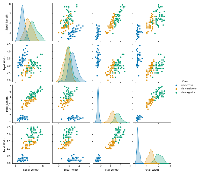
Pairplots of the Iris datasets
This task used the Scikit-learn package to perform the k-means clustering.
For this task I took the following steps:
Gained an overview of how the k-means clustering algorithm works in general
Visualising the Iris dataset
Preprocessing the data including scaling the data, label encoding using sklearn.preprocessing.
Identifying the correct number of clusters using the Elbow method and the Silhouette Scores.
Performing k-means clustering on the data using sklearn.cluster moduel.
Visualising the clusters found using K-means and comparing to the actual Species of Iris.
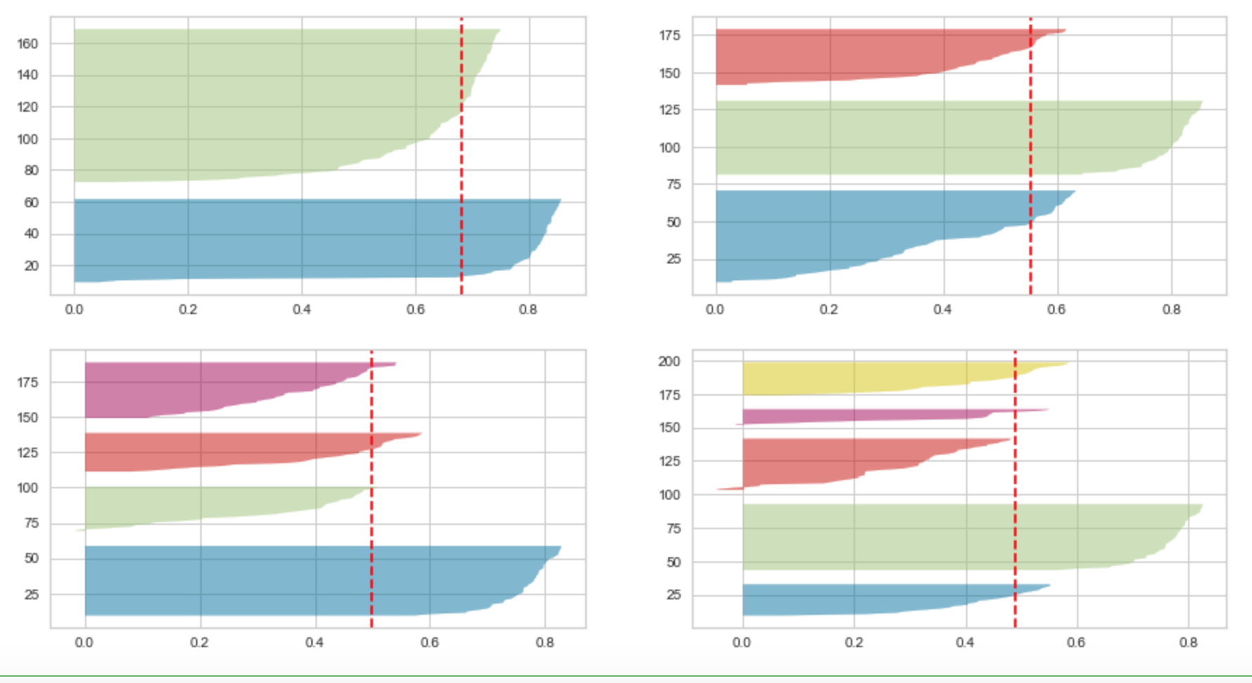
Using the Yellowbrick.cluster library to visualise the Silhouette scores.
Evaluating the performance of the clustering model using Scikit-learns metrics module.
Sihouette Scores using Yellowbrick
Note there was an error in the task instructions as the lecturer meant for us to do K-nearest neighbors instead of K-means clustering.
K-means clustering in an unsupervised learning technique and you do not usually have the labels as you have with the Iris dataset.
K-means is not usually used for making predictions on new data. Unsupervised learning can be used to find patterns in the data or to discover new features.
K-nearest neighbours on the other hand is a supervised learning algorithm that is used for classification and regression. It assumes that similar data points are close to each other.
Nonetheless this gave me an opportunity to learn more about K-means clustering. I will do another notebook on the K-nearest neighbours algorithm which I will include here later.