Machine learning model 1: Polynomial Regression model

The goal of the project is to predict wind power from wind speed and therefore this problem falls into supervised learning. Supervised machine learning is about creating models that precisely map the given inputs (independent variables, or predictors) to the given outputs (dependent variables, or responses).[11]

Regression involves predicting a continuous-valued attribute associated with an object. It is a statistical method used to describe the nature of the relationship between variables which could be positive or negative, linear or nonlinear. Scatter plots visualise a relationship and the correlation coefficient is a measure of the strength of a linear relationship. The correlation statistics show a high correlation between the variables with a value of 0.85. If a scatter plot and the value of the correlation coefficient indicate a linear relationship, the next step is to determine the equation of the regression line which is the data’s line of best fit. Often one of the variables is fixed or controlled and is known as the independent or explanatory variable, the aim is to determine how another variable varies known as the dependent or response variable varies with it. The explanatory variable is usually represented by X while the dependent or response variable is represented by y. Least squares linear regression is a method for predicting the value of a dependent variable y such as power, based on the value of an independent variable x such as wind speeds.

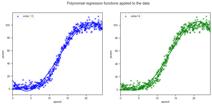
Regression plots were shown above in the exploratory data analysis section, simple linear regression does not adequately model the relationship between the wind and speed values over the entire dataset as there are sections of the datasets that are either above or below the simple linear regression line. The higher order polynomials regression curves have more parameters and do seem to capture more of the relationship between wind speed and power output values. The fourth order polynomial does seem to be even better for the datapoints at the lower end of wind speed values. However it is important not to overfit the data either as then the model will not capture the general trend of the data. There was a suggestion in the research above that an exponent of 3 can be applied to the wind speed factor. [5]. The typical power curves have an s-shape where at wind speeds less than rated the energy capture is approximately proportional to $U^3$ [8] where ($U=\bar{\mu}$) is the 10 minute averaged wind speeds.

For my first machine learning model I will develop two polynomial regression model using the scikit-learn package.

One common pattern within machine learning is to use linear models trained on nonlinear functions of the data. This approach maintains the generally fast performance of linear methods, while allowing them to fit a much wider range of data. [12]

A simple linear regression can be extended by constructing polynomial features from the coefficients. A regression model that is used to model the expected value of a dependent variable y in terms of an independent variable x can be represented by the equation $y=ax+b$. Adding a squared term will create a quadratic model of the form $y=a+b1x+b2^2+e$ where a is the intercept and e is the error rate. Adding a cubed term can be represented by the equation $y=a+b1x+b2x^2+b3x^3+e$. Additional terms can be added. The regression function is linear in terms of the unknown variables and therefore the models are still considered linear from the point of estimation.[15] Scikit-learn’s PolynomialFeatures transforms an input data matrix into a new data matrix of a given degree. Adding an $X^3$ allows us to check if there is a cubic relationship in the data. A polynomial is a special case pf a linear model that is used to fit non-linear data. Adding polynomials to the regression is like multiple linear regression, as you are adding extra variables in the form of powers of each feature as new features. [13]

Regression plots on the cleaned data:

Below are the regression plots using Seaborn regplot function with a 3rd and 4th order applied on the cleaned dataset that excludes some of the zero value observations.

f, axes = plt.subplots(1, 2, figsize=(14, 6))
x = "speed"
y = "power"

sns.regplot(x="speed", y="power", data=dfx, order=3, ax=axes[0], label="order =3", ci=False,marker="x", color="blue"); axes[0].legend()
sns.regplot(x="speed", y="power", data=dfx, order=4, ax=axes[1], label = "order=4",marker='x', color="green"); axes[1].legend()
plt.legend()
plt.suptitle("Polynomial regression functions applied to the data")
plt.savefig("images/Polynomial regression functions.png")

Split data into training and test sets

Splitting your dataset is essential for an unbiased evaluation of prediction performance. The dataset can be split into two or three random subsets.

• A training set: used to train or fit your model. Training set are used to find the optimal weights or coefficients for linear regression, logistic regression, or neural networks.
• A validation set: subset used for unbiased model evaluation during hyperparameter tuning. For each set of hyperparameters, fit the model with the training set and assess it’s performance with the validation set.
• A test set used for an unbiased evaluation of the final model. This should not be used for fitting or validating the model. In less complex cases, when you don’t have to tune hyperparameters, it’s okay to work with only the training and test sets. [11]

Splitting a dataset can also be used for detecting if your model suffers from problems such as underfitting and overfitting.

Underfitting usually arises when a model fails to capture the relationships among data. This can occur when you try to represent non-linear relationships with a linear model. Overfitting occurs when a model has an excessively complex structure and learns both the existing relationships between the variables as well as the noise. Overfitted models usually fail to recognise the general trend of the data. While underfitted models are likely to have poor performance with both the training and testing dataset, overfitted models will usually have strong performance on the training dataset but will have poor performance on the unseen test set. Scikit-learn has a module for splitting the data into training and test sets. The default split is 75% for the training set and 25% for the test set. The random state can be set to make the split reproducible. I initially did not use this but it makes it harder to compare the different machine learning models if you have a different training and test set for each.

Using scikit-learn to split the dataset into training and test subsets:

using sklearn.model_selection.train_test_split

# split into input and output columns

X, y = dfx.values[:, :-1], dfx.values[:, -1:]
# split into train and test datasets
X_train, X_test, y_train, y_test = train_test_split(X, y, test_size=0.25, random_state=0)
print(X_train.shape, X_test.shape, y_train.shape, y_test.shape)
# determine the number of input features

n_features = X_train.shape[1]

(356, 1) (119, 1) (356, 1) (119, 1)

Full dataset df:

To use the full dataset df including the zero power values change uncomment the line below

# split the dataset into input and output columns: df is the full dataset
#X, y = df.values[:, :-1], df.values[:, -1:]

Cleaned dataset dfx:

# split the dataset into input and output columns: dfx is the cleaned dataset
X, y = dfx.values[:, :-1], dfx.values[:, -1:]

# split into train and test datasets
X_train, X_test, y_train, y_test = train_test_split(X, y, test_size=0.25, random_state=0)
print(X_train.shape, X_test.shape, y_train.shape, y_test.shape)
# determine the number of input features
n_features = X_train.shape[1]

(356, 1) (119, 1) (356, 1) (119, 1)

Transform the features of x

Scikit-learns PolynomialFeatures can be used to add a cubic variable or a 4th degree variable to the dataset. Once transformed the new polynomial features can be used with any linear model. The two regression models are developed alongside each other for convenience.

# using scikit-learn, set the order to 3 degrees to include a cubic 
# include_bias=False otherwise I end up with a column of zeros 
poly3 = PolynomialFeatures(degree=3, include_bias=False)
poly4 = PolynomialFeatures(degree=4, include_bias=False)

Note: While working on the web application I came back and updated the model to exclude the constant 1 as an extra term. The model was generating 4 coefficients while I was working with 3 in the web application, the wind speed, wind speed squared and wind speed cubed values. The PolynomialFeatures generate a new feature matrix consisting of all polynomial combinations of the features with degree less than or equal to the specified degree. For example, if an input sample is two dimensional and of the form [a, b], the degree-2 polynomial features are [1, a, b, a^2, ab, b^2]. Therefore I updated the model and set the include_bias to False.

# convert the inputs into a new set of variables, save as X_train_p3 to leave X_train untouched for later use
X_train_poly3 = poly3.fit_transform(X_train)
X_train_poly4 = poly4.fit_transform(X_train)

Look at the new features:

X_train_poly3

array([[8.08300000e+00, 6.53348890e+01, 5.28101908e+02],
       [2.47700000e+00, 6.13552900e+00, 1.51977053e+01],
       [1.57660000e+01, 2.48566756e+02, 3.91890348e+03],
       ...,
       [6.18100000e+00, 3.82047610e+01, 2.36143628e+02],
       [2.25200000e+00, 5.07150400e+00, 1.14210270e+01],
       [9.43400000e+00, 8.90003560e+01, 8.39629359e+02]])

X_train_poly4

array([[8.08300000e+00, 6.53348890e+01, 5.28101908e+02, 4.26864772e+03],
       [2.47700000e+00, 6.13552900e+00, 1.51977053e+01, 3.76447161e+01],
       [1.57660000e+01, 2.48566756e+02, 3.91890348e+03, 6.17854322e+04],
       ...,
       [6.18100000e+00, 3.82047610e+01, 2.36143628e+02, 1.45960376e+03],
       [2.25200000e+00, 5.07150400e+00, 1.14210270e+01, 2.57201528e+01],
       [9.43400000e+00, 8.90003560e+01, 8.39629359e+02, 7.92106337e+03]])

Transform the test sets:

# also need to transform the test data 
X_test_poly3 = poly3.fit_transform(X_test)
X_test_poly4 = poly4.fit_transform(X_test)

Linear regression can now be implemented. This can be thought of as multiple linear regression as new variables in the form of x-squared and x-cubed (and x-quartic?) have been added to the model.

Fitting the model to the training data:

# call the linear regression model
model_poly3 = linear_model.LinearRegression()
model_poly4 = linear_model.LinearRegression()

# fit to the training data
model_poly3.fit(X_train_poly3, y_train)
model_poly4.fit(X_train_poly4, y_train)

LinearRegression()

Predict using the polynomial regression model:

# predict on the transformed test data
poly3_predictions = model_poly3.predict(X_test_poly3)
poly4_predictions = model_poly4.predict(X_test_poly4)

# Predicting a new result with Polymonial Regression
model_poly3.predict(poly3.fit_transform([[0]]))

array([[14.35877751]])

# Predicting a new result with Polymonial Regression
model_poly4.predict(poly4.fit_transform([[0]]))

array([[9.94417577]])

model_poly3.predict(poly3.fit_transform([[12]]))

array([[45.01454843]])

# Predicting a new result with Polymonial Regression
model_poly4.predict(poly4.fit_transform([[12]]))

array([[43.28996568]])

Get the coefficients

# get the coefficiets
model_poly3.coef_

array([[-9.69965794,  1.49732   , -0.03967732]])

# get the coefficiets
model_poly4.coef_

array([[-5.98949605e+00,  8.11385527e-01,  3.98058010e-03,
        -8.92082165e-04]])

# get the intercept
model_poly3.intercept_

array([14.35877751])

# get the intercept
model_poly4.intercept_

array([9.94417577])

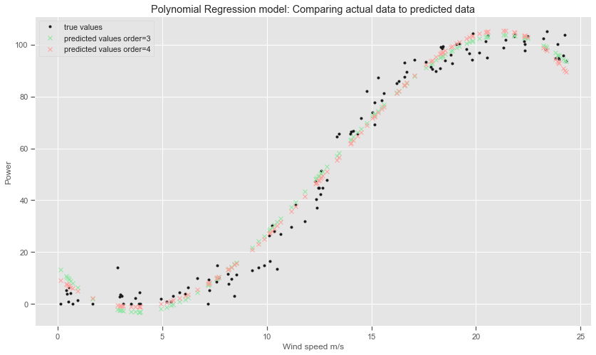
Visualise the Polynomial Regression results:

The scatter-plot can visualise the polynomial regression results on the test dataset can compared to the actual datapoints.

# create the plot
plt.style.use('ggplot')
# Plot size.
plt.rcParams['figure.figsize'] = (14, 8)
plt.title('Polynomial Regression model: Comparing actual data to predicted data')
plt.plot(X_test, y_test, 'k.', label="true values")
plt.plot(X_test, poly3_predictions, 'gx', label="predicted values order=3")
plt.plot(X_test, poly4_predictions, 'rx', label="predicted values order=4")
plt.xlabel("Wind speed m/s")
plt.ylabel("Power")
plt.legend()

plt.savefig("images/Polynomial Regression Model: Comparing actual data to predicted data")

Evaluate the Polynomial Regression model:

Scikit-learn has a metrics module sklearn.metrics that can be used to evaluate the models.

The coefficient of determination $R^2$ is the proportion of the variance in the dependent variable that is predictable from the independent variable(s).[16] It shows how good the model is at explaining the behaviour of the dependent variable. The coefficient of determination is the proportion of variation in the dependent variable power that is explained by the regression line and the independent variable wind speed. It is a better indicator of the strength of a linear relationship than the correlation coefficient as it identifies the percentage of variation of the dependent variable that is directly attributable to the variation of the independent variable.

The model can be evaluated using the mean squared error. It calculates the average distance our data points are from the model.
The mean squared error could be further lowered by adding extra polynomials to the model. However you are then in danger of overfitting the model where the model will fail to recognise the general trend. The simple linear model cleared underfit the data. The Seaborn regression plots with a 4th order polynomial earlier did show a slightly better fit for speed values under 5 metres per second whereas the 3rd order polynomial is underpredicting and overfitting for sections of the curve. Polynomial regression can be very sensitive to outliers and even a few outliers could seriously affect the results. In addition there are unfortunately fewer model validation tools for the detection of outliers in nonlinear regression than there are for linear regression. [16]

The root mean squared error is the square root of the average of squared differences between prediction and actual observation. It is a standard way to measure the error of a model in predicting quantitative data.

from sklearn.metrics import mean_squared_error, r2_score

# The coefficients
print('Coefficients: \n', model_poly3.coef_)

Coefficients: 
 [[-9.69965794  1.49732    -0.03967732]]

$R^2$ and RMSE for the 3rd order Polynomial Regression model:

print("Results from 3rd degree polynomial regression:")
print('Mean squared error: %.2f' % mean_squared_error(y_test,poly3_predictions ))
# The coefficient of determination: 1 is perfect prediction
print('Coefficient of determination: %.2f' % r2_score(y_test, poly3_predictions))
print('Root Mean Squared Error: %.2f' % np.sqrt(mean_squared_error(y_test,poly3_predictions )))

Results from 3rd degree polynomial regression:
Mean squared error: 33.32
Coefficient of determination: 0.98
Root Mean Squared Error: 5.77

$R^2$ and RMSE for the 4th order Polynomial Regression model:

print("Results from 4th degree polynomial regression:")
print('Mean squared error: %.2f' % mean_squared_error(y_test,poly4_predictions ))
# The coefficient of determination: 1 is perfect prediction
print('Coefficient of determination: %.2f' % r2_score(y_test, poly4_predictions))
print('Root Mean Squared Error: %.2f' % np.sqrt(mean_squared_error(y_test,poly4_predictions )))

Results from 4th degree polynomial regression:
Mean squared error: 30.80
Coefficient of determination: 0.98
Root Mean Squared Error: 5.55

The mean squared error for the 4th order polynomial did fall a little compared to the polynomial using 3 degrees. The R-squared value does not seem to have changed much though. The curves above show that they both overestimate the power values for very low wind speed values. For the slightly higher wind speed values the curve predicts negative values of power. Fitting higher order polynomials might pick up more of the trends in the training data but would be unlikely to work very well with new data.

Predict using the polynomial regression models:

# Predicting a new result with Polymonial Regression
# need to transform the data to be predicted
model_poly3.predict(poly3.fit_transform([[20]]))

array([[101.8750371]])

# need to transform the data to be predicted
model_poly4.predict(poly4.fit_transform([[20]]))

array([[103.81995991]])

# Predicting a new result with Polymonial Regression
model_poly3.predict(poly3.fit_transform([[24.4]]))

array([[92.74766278]])

# Predicting a new result with Polymonial Regression
model_poly3.predict(poly3.fit_transform([[3]]))

array([[-2.33560405]])

Save the model for use in the Web application

This project also requires a web service to be developed that will respond with predicted power values based on speed values sent as HTTP requests. Therefore I need to save the model for use outside this notebook.

For the polynomial regression model, there is the option of using Python’s built-in persistence model pickle. The scikit-learn documents recommend using joblib’s replacement of pickle (dump & load), which is more efficient on objects that carry large numpy arrays internally as is often the case for fitted scikit-learn estimators, but can only pickle to the disk and not to a string.

The models are saved in a folder called models in this repository. The code here can be uncommented to save the models again.

#from joblib import dump, load
#dump(model_poly3, 'models/model_poly3.joblib') 
#dump(model_poly4, 'models/model_poly4.joblib') 

#dump(model_poly3, 'models/model_poly3.pkl') 
#dump(model_poly4, 'models/model_poly4.pkl') 

wind12 = poly3.fit_transform([[12]])
wind12

array([[  12.,  144., 1728.]])

windp4_12 = poly4.fit_transform([[12]])
windp4_12

array([[1.2000e+01, 1.4400e+02, 1.7280e+03, 2.0736e+04]])

model_poly4.predict(windp4_12)

array([[43.28996568]])

wind12 = [[12, 12**2, 12**3]]
wind12 =np.array(wind12)

model_poly3.predict(wind12)

array([[45.01454843]])

wind3 = [[3, 3**2, 3**3]]
wind3 = np.array(wind3)
model_poly3.predict(wind3)

array([[-2.33560405]])

Some notes on the Polynomial Regression models:

While the Polynomial regression model does quite a good job, it predicts power values for values over 24.4 which is the cut-off range. The transformations have also to be taken into account when taking in new values from the end user.