Machine Learning Model 2: Artificial Neural Network
For my second machine learning model I will implement an Artificial Neural Network using the tf.keras API.
In addition to the lecture videos I followed several tutorials in particular those by MachineLearningMastery.com [20] as well as the Tensorflow-Keras documentation and other tutorials documented in the references section below. TensorFlow is the premier open-source deep learning framework developed and maintained by Google. Keras is a deep learning API written in Python, running on top of the machine learning platform TensorFlow.[21]
A Multilayer Perceptron model (MLP) is a standard fully connected Neural Network model. It is made up of one or more (dense) layers of nodes where each node is connected to all outputs from the previous layer and the output of each node is connected to all the inputs for the nodes in the next layer. This model is suitable for tabular data and can be used for three predictive modeling problems being binary classification, multiclass classification, and regression.[20]
Machine learning is the science of getting computers to act without being explicitly programmed. Artificial neural networks are a class of machine-learning algorithms that are used to model complex patterns in datasets through the use of multiple hidden layers and non-linear activation functions. They are designed to simulate the way the human brain analyses and processes information. The computer learns to perform some task by analyzing training examples.
An artificial neural network (ANN) is the piece of a computing system designed to simulate the way the human brain analyzes and processes information. It is the foundation of artificial intelligence (AI) and solves problems that would prove impossible or difficult by human or statistical standards. ANNs have self-learning capabilities that enable them to produce better results as more data becomes available.[17]
Neural nets are a means of doing machine learning, in which a computer learns to perform some task by analyzing training examples. Modeled loosely on the human brain, a neural net consists of thousands or even millions of simple processing nodes that are densely interconnected. Most of today’s neural nets are organized into layers of nodes, and they’re “feed-forward,” meaning that data moves through them in only one direction. An individual node might be connected to several nodes in the layer beneath it, from which it receives data, and several nodes in the layer above it, to which it sends data. To each of its incoming connections, a node will assign a number known as a “weight.” When the network is active, the node receives a different data item — a different number — over each of its connections and multiplies it by the associated weight. It then adds the resulting products together, yielding a single number. If that number is below a threshold value, the node passes no data to the next layer. If the number exceeds the threshold value, the node “fires,” which in today’s neural nets generally means sending the number — the sum of the weighted inputs — along all its outgoing connections. When a neural net is being trained, all of its weights and thresholds are initially set to random values. Training data is fed to the bottom layer — the input layer — and it passes through the succeeding layers, getting multiplied and added together in complex ways, until it finally arrives, radically transformed, at the output layer. During training, the weights and thresholds are continually adjusted until training data with the same labels consistently yield similar outputs.[18]
A neural network takes an input and passes it through multiple layers of hidden neurons. These hidden neurons can be considered as mini-functions with coefficients that the model must learn. The neural network will output a prediction that represents the combined input of all the neurons. Neural networks are trained iteratively using optimization techniques such as gradient descent.
After each cycle of training, an error metric is calculated based on the difference between the prediction and the target. The derivatives of this error metric are calculated and propagated back through the network using a technique called backpropagation. Each neuron’s coefficients (weights) are then adjusted relative to how much they contributed to the total error. This process is repeated iteratively until the network error drops below an acceptable threshold. [19]
To use artificial neural networks on a dataset all variables need to be first encoded into floating point numbers. Outputs can be reverse decoded later. A neuron takes a group of weighted inputs, applies an activation function and returns an output. The inputs to a neuron can be features from a training set or the outputs from the previous layer’s neurons. The weights and bias are the parameters of the model. The initial weights are often set to small random values and can be adjusted to get the neural network to perform better. Weights are applied along the inputs as they travel along the ‘synapses’ (the connection between two neurons) to reach the neuron. The neuron then applies an activation function to the sum of the weighted inputs from each incoming synapse and passes the result to all the neurons in the next layer. Weights are applied to each connection. These are values that control the strength of the connection between two neurons. Inputs are usually multiplied by weight that define how much influence the input will have on the output. The lower the weight the lower the importance of the connection while the higher the weight the higher the importance of the connection. When the inputs are transmitted between the neurons, the weights are applied to the inputs as well as an additional value known as the bias. The bias are additional constant terms that are attached to each neuron and are added to the weighted input before the activation function is applied. Bias terms help models represent patterns that do not necessarily pass through the origin. [19] Bias terms must also be learned by the model.
The input layer of a neural network will hold the data to train the model. Neural networks can have several input features each represented by a neuron that represents the unique attributes in the dataset. This dataset has a single input feature, the wind speed in metres per second.
The neural network can have one or more hidden layers between the input layer and the output layer. The hidden layers applies an activation function before passing on the results to the next layer. Hidden layers can be fully connected or dense layers where each neuron receives inputs from all the neurons in the previous layer and sends its output to each neuron in the next layer. Alternatively with a convolutional layer the neurons will send their output to only some of the neurons in the next layer. The output layer is the final layer in the neural network and receives its input from the previous hidden layer. It can also apply an activation function and returns an output. The output represents the prediction from the neural network.
With neural networks the aim is to get a high value assigned to the correct output. If the neural network misclassifies an output label then it is fed back into the algorithm, the weights are changed a little so that the correct output is predicted the next time and this will keep changing until it gets the correct output.
The starting values for the weights are usually random values and which updated over time to achieve the expected output using an algorithm such as gradient descent (or stochastic gradient descent sgd) or some other algorithm.
The input to a neuron is the sum of the weighted outputs from all the neurons in the previous layer. Each input is multiplied by the weight associated with the synapse or connnection connecting the input to the current neuron.
If there are n inputs or neurons in the previous layer then each neuron in the current layer will have n distinct weight with one weight for each connection.
For multiple inputs this is $x_1w_1+x_2w_2+x_3w_3$ which is the same equation as used for linear equation. A neural network with a single neuron is actually the same as linear regression except that the neural network post-processes the weighted inputs with an activation function. [19]
There are activation function inside each layer of a neural network which modifies the inputs they receive before passing them onto the next layer. Activation functions allow a neural network to model complex non-linear functions. In order to be able to use gradient descent the outputs need to have a slope with which to calculate the error derivative with respect to the weights. If the neuron only outputted a 0 or 1 then this doesn’t tell us in what direction the weights need to be updated to reduce the error.
An article on Medium.com [22] provides some background on activation functions which I refer to here: An artificial neuron calculates a weighted sum of its input, adds a bias and then decides whether it should be fired or not. $Y = \sum{(\text{weight} * \text{input})} + \text{bias}$. The value of Y can be anything from -infinity to + infinity and the neuron does not really know the bounds of the value. To decide whether the neuron should fire or not the activation function checks the $Y$ value produced by the neuron and decides whether outside connections should consider this neuron as activated (fired) or not. With a threshold based activation function, if the value of Y is above a certain value then it can be declared as activated and otherwise not. The output is 1 (activated) when the value is greater than the threshold and 0 otherwise. This is a step function which has drawbacks being used as an activation function when the response is not a binary yes or no. A linear activation function $A=cX$ is a straight line function where activation is proportional to input (which is the weighted sum from neurons). In this way it will give a range of activations rather than just binary activations. Nuerons can be connected and if more than one fire then you can take the max and make a decision based on that. The derivative w.r.x is c which means that the gradient has no relationship with X. The descent is going to be on a constant gradient. If there is an error in prediction the changes made by back propagation is constant and not depending on the change in input delta(x). Another problem concerns the connected layers where each layer is activated by a linear function. That activation in turn goes into the next level as input and the second layer calculates weighted sum on that input and it in turn, fires based on another linear activation function. No matter how many layers we have, if all are linear in nature, the final activation function of last layer is nothing but just a linear function of the input of first layer. Therefore two or more layers can be replaced by a single layer. The whole network then is equivalent to a single layer with linear activation.
The sigmoid function is smooth and looks somewhat like a step function. It is nonlinear in nature and therefore combinations of layers are also non-linear which means that layers can be stacked. It will also give non-binary activations unlike the step function. It has a smooth gradient. Between X values -2 to 2, the Y values are very steep. This means that any small changes in the values of X in that region will cause values of Y to change significantly. This means this function has a tendency to bring the Y values to either end of the curve. It tends to bring the activations to either side of the curve making clear distinctions on prediction. Another advantage over linear function is that the output of the activation function is always going to be in range (0,1) compared to (-inf, inf) of linear function and therefore the activations are bound in a range. Sigmoid functions are one of the most widely used activation functions today. The problems with them is that towards either end of the sigmoid function, the Y values tend to respond less to changes in X. This means that the gradient at that region is going to be small. It gives rise to a problem of “vanishing gradients”. When the activations reach near the “near-horizontal” part of the curve on either sides, the gradient is small or has vanished (cannot make significant change because of the extremely small value). The network refuses to learn further or is drastically slow (depending on use case and until gradient /computation gets hit by floating point value limits ). There are ways to work around this problem and sigmoid is still very popular in classification problems. The same article also looked at the Tanh activation functions which is a scaled sigmoid function and the ReLu function which gives an output x if x is positive and 0 otherwise. These are both non-linear functions. The article also suggested how to choose the correct activation function for your model. When you know the function you are trying to approximate has certain characteristics, you can choose an activation function which will approximate the function faster leading to faster training process.
The loss function or cost function tells us how well the model predicts for a given set of parameters. It has its own curve and derivative and the slope of this curve informs how to change the parameters to make the model more accurate. The lost or cost functions for regression problems is usually the mean squared error MSE. Other loss functions would be used for classification problems.
Once the neural network is trained and is stable, if a new datapoint that it was not trained on is provided to it the neural network should be able to correctly classify it.
Developing Machine Learning Model 2: An Artificial Neural Network
The data:
I am using the dataframe dfx where some of the zero values were dropped.
I can alternatively try using the df dataframe consisting of all 500 rows.
dfx.describe()
.dataframe tbody tr th {
    vertical-align: top;
}

.dataframe thead th {
    text-align: right;
}
Split the data into training and test sets
The ideal machine-learning model is end to end and therefore the preprocessing should be part of the model as much as possible to make the model portable for production. However I have already split the dataset earlier for the polynomial regression model and need to be able to compare the models.
dfx.values.shape
(475, 2)
# split into input and output columns

X, y = dfx.values[:, :-1], dfx.values[:, -1:]
# split into train and test datasets
X_train, X_test, y_train, y_test = train_test_split(X, y, test_size=0.25, random_state=0)
print(X_train.shape, X_test.shape, y_train.shape, y_test.shape)
# determine the number of input features

n_features = X_train.shape[1]
(356, 1) (119, 1) (356, 1) (119, 1)
print(X_train.shape, X_test.shape, y_train.shape, y_test.shape)
# determine the number of input features
n_features = X_train.shape[1]
(356, 1) (119, 1) (356, 1) (119, 1)
Full dataset df:
To apply the model to the full dataset uncomment the code below.
# split the dataset into input and output columns: df is the full dataset
#X, y = df.values[:, :-1], df.values[:, -1:]
# split into train and test datasets
#X_train, X_test, y_train, y_test = train_test_split(X, y, test_size=0.25, random_state=0)
#print(X_train.shape, X_test.shape, y_train.shape, y_test.shape)
# determine the number of input features
#n_features = X_train.shape[1]
# split the dataset into input and output columns: df is the full dataset
#X, y = df.values[:, :-1], df.values[:, -1:]
To normalise or not.
The Introduction to Keras for Engineers does suggest that data preprocessing should be done such as feature normalisation. Normalization is a rescaling of the data from the original range so that all values are within the range of 0 and 1. According to the tutorial the data should either be rescaled to have zero-mean and unit-variance or the data in the [0.1] range. The preprocessing should ideally be done as part of the model to make it more portable in production. In Keras the preprocessing is done via preprocessing layers which can be included directly into your model either during training or after training.
Normalization should be done after splitting the data into train and test/validation to avoid data leakage. This is where information from outside the dataset is used to train the model. Normalization across instances should be done using only the data from the training set. Using any information coming from the test set before or during training is a potential bias in the evaluation of the performance.
I initially followed some tutorials that used scikit-learn package for scaling or normalising data but then realised that this would be a problem on the web application side as the data taken in would have to have the same scaling or normalisation applied as the training data. Keras does have some preprocessing layers including the Normalization layer for feature normalization.
Many examples in blogs and tutorials only scale the inputs or the target variable but in this dataset we only have a single numerical input variable and a single numerical target variable. The values for wind speed and power output in this dataset do not have very different scales.
Without scaling the model does quite a good job considering all it has are these two single columns of numbers.
A machine learning model has a life-cycle with 5 steps:[20]
1. Define the model:
Select the type of model and choose the architecture or network topology. Define the number of layers, configure each layer with a number of nodes and activation function, connect the layers together into a cohesive model. A layer is a simple input-output transformation while a model is a directed acyclic graph of layers. It is like a bigger layer consisting of many sub-layers that can be trained via exposure to data. According to any tutorials I came across, determining the correct number of layers to use is a matter of trial and error really. Generally you need a network large enough to capture the structure of the problem.
The input layer is first defined, then you chain layer transformations on top of the inputs until the final output.
All layers in Keras need to know the shape of their inputs in order to be able to create weights. The shape of the weights depends on the shape of their inputs. The Input object is not considerd a layer.
The visible layer of the network is defined by the input shape argument on the first hidden layer. In the dataset for this project this will be (1,) as there is only a single input variable wind speed. The model will then expect the input for one sample to be a vector of 1 number.
There are two main models that are provided in the tensorflow-keras API. A Sequential model is appropriate for a plain stack of layers where each layer has exactly one input tensor and one output tensor. A Sequential model is not appropriate for models with multiple inputs or outputs. A sequential neural network is built up in sequential layers. It adds layers to the model one by one in a linear manner, from input to output. I will be using the Sequential model for this project. A Sequential model is created by passing a list of layers to the Sequential constructor model = keras.Sequential or by incrementally adding the layers using the model.add() method.
There is also a Functional model which is more complex but more flexible than the Sequential model. For this you need to explicitly connect the output of one layer to the input of another layer. Each connection is specified.
Fully connected layers are defined using the Dense class - Dense refers to the layer being densely connected to the previous layer. Every node in the previous layer is connected to everything in the current layer.
The first line of code that adds the first Dense layer does 2 things, defines the input or visible layer and the first hidden layer. The number of neurons or nodes in the layer as the first argument and specify the activation function using the activation argument. We were advised to use the Sigmoid activation function for this project so I will do this. A Sigmoid layer is used on the outer layer to ensure the network output is between 0 and 1.
According to the tutorials, Sigmoid and Tanh activation functions were the preferred choice for all layers before but that these days better performance is achieved using the rectified linear unit or ReLU activation function.
Initializers define the way to set the initial random weights of Keras layers. The kernel_initializer and bias_initializer parameter refers to the distribution or function to use for initialising the weights. Initializers available include RandomNormal class , RandomUniform class, a Zeros class, a Ones class. GlorotNormal draws samples from a truncated normal distribution centered on 0. GlorotUniform draws samples from a uniform distribution within some limits.
Once the layers have been defined that turn the inputs into outputs, instantiate a model object.
# Define a model
model = kr.models.Sequential()
# Here I played around with the kernel initialiser but it did not do much good
initializer = kr.initializers.RandomUniform(minval=0., maxval=24.4)
model.add(kr.layers.Dense(20, input_shape=(1,), activation='sigmoid', kernel_initializer=initializer, bias_initializer="glorot_uniform"))
model.add(kr.layers.Dense(20, input_shape=(1,), activation='sigmoid', kernel_initializer="glorot_uniform", bias_initializer="glorot_uniform"))
model.add(kr.layers.Dense(1, activation='linear', kernel_initializer="glorot_uniform", bias_initializer="glorot_uniform"))
2. Compile the model
Once the model is defined, it can be compiled or built using the compile() method passing in the selected loss functions and optimizer functions. For this project I use the mean squared error as the cost function as this is a regression problem.
Loss functions such as MeanSquaredError computes the mean of squares of errors between labels and predictions.
There are many more listed in the keras losses documentation.
The optimizer performs the optimisation procedure such as stochastic gradient descent or Adam . Adam is a modern variation of stochastic gradient descent method which automatically tunes itself and gives good results in a wide range of problems. The optimizer can be specified as a string for a known optimizer class such as sgd for stochastic gradient descent or else you can configure an instance of the optimizer classes to use.
sgd is a gradient descent (with momentum) optimizer. It has a default learning rate of 0.01
The update rule is w = w - learning_rate * g for parameter w with gradient g when momentum is 0.
The learning_rate defaults to 0.001 in the Adam optimizer.
You can also select some performance metrics to keep track of and report during the model training process.
Metrics to evaluate predictions from the model include Accuracy to calculates how often predictions equal labels, AUC computes the approximate area under the curve, FalseNegatives calculates the number of false negatives and FalsePositives calculates the number of false positives, Precision computes the precision of the predictions with respect to the labels.
#
model.compile(kr.optimizers.Adam(lr=0.001), loss='mean_squared_error')
model.summary()
Model: "sequential"
_________________________________________________________________
Layer (type)                 Output Shape              Param #
=================================================================
dense (Dense)                (None, 20)                40
_________________________________________________________________
dense_1 (Dense)              (None, 20)                420
_________________________________________________________________
dense_2 (Dense)              (None, 1)                 21
=================================================================
Total params: 481
Trainable params: 481
Non-trainable params: 0
_________________________________________________________________
3. Fit the model
- Once the model has been compiled, fit the model to the data using
fit(). To fit the model you need to select the training configuration such as the number of epochs which are loops or iterations through the training dataset. The batch size is the number of samples in an epoch used to estimate model error. By passing in for example 10 at a time instead of 1 at a time can have a smoothing effect.
Training applies the chosen optimization algorithm to minimize the chosen loss function and updates the model using the backpropagation of error algorithm. This can be slow depending on the complexity of the model, the size of the training dataset and the hardware being used.
The fit call returns a history object which records what happens over the course of the training.
- The
history.historydict contains per-epoch timeseries of metrics values. - Validation data can be passed to
fit()to monitor the validation loss & validation metrics which get reported at the end of each epoch.
When passing data to the built-in training loops of a model, NumPy arrays can be used if the data is small and fits in memory or tf.data.Dataset objects. The dataset here is only 500 rows.
Training the model on the training data:
# fit the model

#history=model.fit(X_train, y_train, validation_data =(X_test, y_test),epochs=500, batch_size=10) #verbose=0
history = model.fit(X_train, y_train, epochs=500, batch_size=10, validation_split=0.2)
See code output 1 for full output.
Epoch 1/500
     1/29 [>.............................] - ETA: 0s - loss: 5701.8042WARNING:tensorflow:Callbacks method `on_train_batch_end` is slow compared to the batch time (batch time: 0.0010s vs `on_train_batch_end` time: 0.0018s). Check your callbacks.
    29/29 [==============================] - 0s 11ms/step - loss: 3915.3535 - val_loss: 3900.9231
    Epoch 2/500
    29/29 [==============================] - 0s 4ms/step - loss: 3840.3071 - val_loss: 3829.6680
    Epoch 3/500
    Epoch 495/500
    29/29 [==============================] - 0s 2ms/step - loss: 17.0002 - val_loss: 15.8715
    Epoch 496/500
    29/29 [==============================] - 0s 2ms/step - loss: 17.1516 - val_loss: 15.9868
    Epoch 497/500
    29/29 [==============================] - 0s 5ms/step - loss: 17.1033 - val_loss: 15.7123
    Epoch 498/500
    29/29 [==============================] - 0s 2ms/step - loss: 16.9916 - val_loss: 15.7983
    Epoch 499/500
    29/29 [==============================] - 0s 2ms/step - loss: 17.1141 - val_loss: 15.7787
    Epoch 500/500
    29/29 [==============================] - 0s 2ms/step - loss: 17.5874 - val_loss: 16.1258
4. Evaluating the model:
After fit() you can evaluate the performance and generate predictions on new data using evaluate().
This is where the holdout dataset comes into play, data that is not used in the training of the model so you can get an unbiased estimate of the performance of the model when making predictions on new data.
Plotting the learning curve:
You can also plot the model learning curves which plot the performance of the neural network model over time. It helps determine if the model is learning well and whether it is underfitting or overfitting the training set. To do this you need to update the call to to the fit function to include a reference to a validation dataset which is a portion of the training dataset not used to fit the model but instead used to evaluate the performance of the model during training. The fit function will then return a history object containing a trace of performance metrics recorded at the end of each training epoch. A learning curve is a plot of the loss on the training dataset and the validation dataset.
Learning curves of mean squared error on the train and test set at the end of each training epoch are graphed below using line plots. These learning curves give an indication of the dynamics while learning the model.
The learning curve below shows that the loss from the validation data is very close to the loss from the training data. This can also be seen by the print outs for each epoch above. The loss falls dramatically over the first 100 epochs and then the decrease stabilises.
#history = model.fit(X_train, y_train, epochs=500, batch_size=10, verbose=0, validation_split=0.3)
plt.title('Learning Curves for a Neural Network')
plt.xlabel('Epoch')
plt.ylabel('Mean Squared Error')
plt.plot(history.history['loss'], 'r.',label='train')
plt.plot(history.history['val_loss'], 'b.',label='validation')
plt.legend()
plt.savefig("images/Neural Network Learning curves")
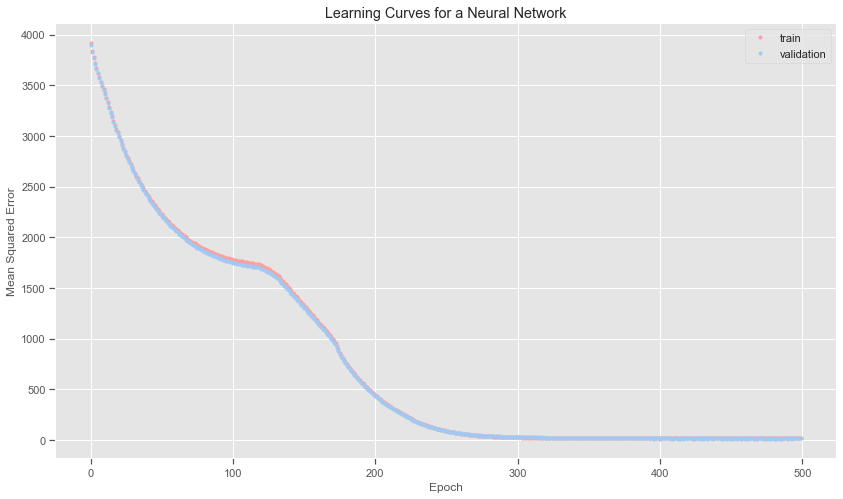
The ideal loss is is zero and the ideal accuracy is 1.0 or 100%. The root mean squared error is quite low overall. The loss is slightly higher though on the test set than on the training data. However over almost 500 data point this does not seem too bad at all.
Evaluate() the performance of the model on new data:
train_mse = model.evaluate(X_train, y_train, verbose=0)
test_mse = model.evaluate(X_test, y_test, verbose=0)
print('Train MSE: %.3f, Test MSE: %.3f' % (train_mse, test_mse))
Train MSE: 16.753, Test MSE: 17.035
train_rmse = np.sqrt(train_mse)
test_rmse = np.sqrt(test_mse)
print('Training data RMSE: %.3f, Test data RMSE: %.3f' % (train_rmse, test_rmse))
Training data RMSE: 4.093, Test data RMSE: 4.127
5. Make predictions using the neural network model
This is the final stage of the life cycle where you take values that you don’t have target values and make a prediction using the model
- Generate numPy arrays of predictions using
predict().predictions = model.predict(val_dataset)
Predictions using the neural network model:
Run each x value through the neural network.
model_predictions = model.predict(X_test)
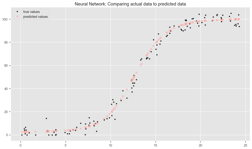
Compare actual data to predictions on test set
plt.style.use('seaborn-colorblind')
plt.title('Neural Network: Comparing actual data to predicted data')
plt.plot(X_test, y_test, 'k.', label="true values")
plt.plot(X_test, model_predictions, 'rx', label="predicted values")

plt.legend()
plt.savefig("images/Neural Network: Comparing actual data to predicted data")
#model.predict([0])
#model.predict([24.5])
Notes on the neural network model:
The neural network model is over-predicting the power value when the wind speed exceeds the cut-off rates. I guess the model does not actually know this bit of information! I removed these observations from the training data as the dataset and research suggests that than for safety reasons the turbines are turned off when wind speed exceeds 24.4 metres per second. I need to take this into account in the prediction web service application. The neural network model is also predicting power values when the wind speed is zero. This is not really a problem as you would not expect to be predicting the power output for non-existent wind. I did try adding extra layers and playing around with the parameters but to no avail. This makes the model more computationally expensive.
Overall the model is better at predicting power for the lower values of wind speed than the polynomial regression models. The plot shows that the predictions go right through the test data points and captures the overall trend.
I did change the kernel_initializer to random_uniform and specified a min and max values in the first hidden layer as I thought this might help but the model still predicts a non-zero values for zero wind speeds and for speeds greater than the cut-off wind speed of 24.4 metres per second. I need to know some more about how the kernel initialisers actually work.
#model.predict([26])
#model.predict([23.5])
#model.predict([0])
#model.predict([12])
Save the model for use in the web application:
Instead of having to retrain the model each time, it can be saved to a file using the save() function on the model and loaded later to make predictions using the load_model() function. The model is saved in H5 format, an efficient array storage format. For this I need the h5py library.
#model.save('models/model.h5')
Some variations of the same artificial neural network model:
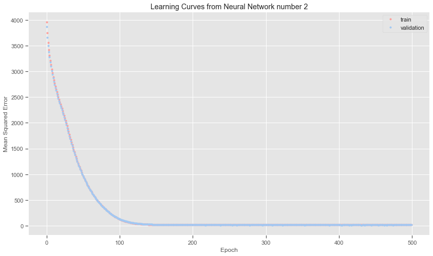
Here I tried out changing the kernel_initialiser to using the glorot_uniform initialiser. More neurons were added in the second layer. The loss does fall quicker as can be seen from the printouts as well as the learning curve. The difference in cost between the different versions of the neural network models is very small. It does seem as if all roads lead to Rome!
Define a model:
# Define a model
model2 = kr.models.Sequential()

model2.add(kr.layers.Dense(50, input_shape=(1,), activation='sigmoid', kernel_initializer="glorot_uniform", bias_initializer="glorot_uniform"))

model2.add(kr.layers.Dense(50, input_shape=(1,), activation='sigmoid', kernel_initializer="glorot_uniform", bias_initializer="glorot_uniform"))
model2.add(kr.layers.Dense(1, activation='linear', kernel_initializer="glorot_uniform", bias_initializer="glorot_uniform"))
Compile the model:
# compile the model
model2.compile(kr.optimizers.Adam(lr=0.001), loss='mean_squared_error')
model2.summary()
Model: "sequential_1"
_________________________________________________________________
Layer (type)                 Output Shape              Param #
=================================================================
dense_3 (Dense)              (None, 50)                100
_________________________________________________________________
dense_4 (Dense)              (None, 50)                2550
_________________________________________________________________
dense_5 (Dense)              (None, 1)                 51
=================================================================
Total params: 2,701
Trainable params: 2,701
Non-trainable params: 0
_________________________________________________________________
Fit a model:
history2=model2.fit(X_train, y_train, validation_split=0.2,epochs=500, batch_size=10) #verbose=0
Epoch 1/500
    29/29 [==============================] - 0s 8ms/step - loss: 3957.2795 - val_loss: 3869.7856
    Epoch 2/500
    29/29 [==============================] - 0s 3ms/step - loss: 3745.3003 - val_loss: 3663.5308
    Epoch 3/500
    29/29 [==============================] - 0s 2ms/step - loss: 3561.5083 - val_loss: 3500.2002
    Epoch 4/500
    29/29 [==============================] - 0s 4ms/step - loss: 3419.5115 - val_loss: 3376.7346
    Epoch 5/500
  Epoch 497/500
    29/29 [==============================] - 0s 2ms/step - loss: 16.8655 - val_loss: 15.3804
    Epoch 498/500
    29/29 [==============================] - 0s 2ms/step - loss: 16.8284 - val_loss: 15.7348
    Epoch 499/500
    29/29 [==============================] - 0s 2ms/step - loss: 16.9639 - val_loss: 15.3813
    Epoch 500/500
    29/29 [==============================] - 0s 2ms/step - loss: 17.1498 - val_loss: 17.0126
Evaluate the model
#history = model.fit(X_train, y_train, epochs=500, batch_size=10, verbose=0, validation_split=0.3)
plt.title('Learning Curves from Neural Network number 2')
plt.xlabel('Epoch')
plt.ylabel('Mean Squared Error')
plt.plot(history2.history['loss'], 'r.',label='train')
plt.plot(history2.history['val_loss'], 'b.',label='validation')
plt.legend()
plt.savefig("images/Learning Curves from Neural Network number 2'")
# Evaluate the model
print("Evaluating Neural Network Model number 2:")
train_mse2 = model2.evaluate(X_train, y_train, verbose=0)
test_mse2 = model2.evaluate(X_test, y_test, verbose=0)
print('Train MSE: %.3f, Test MSE: %.3f' % (train_mse2, test_mse2))

train_rmse2 = np.sqrt(train_mse2)
test_rmse2 = np.sqrt(test_mse2)
print('Training data RMSE: %.3f, Test data RMSE: %.3f' % (train_rmse2, test_rmse2))
Evaluating Neural Network Model number 2:
Train MSE: 16.822, Test MSE: 18.529
Training data RMSE: 4.101, Test data RMSE: 4.305
Predictions with this neural network model:
model2_predictions = model2.predict(X_test)
#model2.save('models/model2.h5')
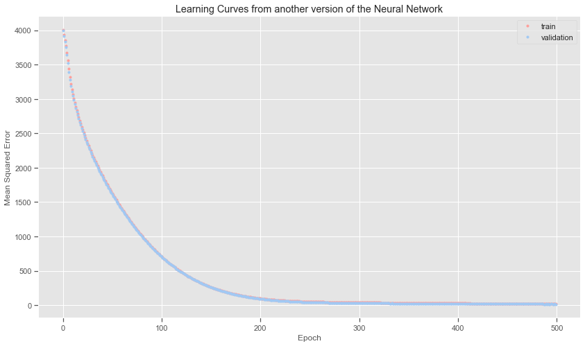
Reduce the number of layers in the Neural Network:
Here I am just seeing how reducing the number of layers and the number of neurons will affect the final results.
Define another neural network model:
# define a model
model3 = kr.models.Sequential()

model3.add(kr.layers.Dense(30, input_shape=(1,), activation='sigmoid', kernel_initializer="glorot_uniform", bias_initializer="glorot_uniform"))


model3.add(kr.layers.Dense(1, activation='linear', kernel_initializer="glorot_uniform", bias_initializer="glorot_uniform"))
Compile the neural network model:
# compile the model
model3.compile(kr.optimizers.Adam(lr=0.001), loss='mean_squared_error')
model3.summary()
Model: "sequential_2"
_________________________________________________________________
Layer (type)                 Output Shape              Param #
=================================================================
dense_6 (Dense)              (None, 30)                60
_________________________________________________________________
dense_7 (Dense)              (None, 1)                 31
=================================================================
Total params: 91
Trainable params: 91
Non-trainable params: 0
_________________________________________________________________
Fit the neural network model:
# fit the model
history3=model3.fit(X_train, y_train, validation_split=0.2,epochs=500, batch_size=10) #verbose=0
    Epoch 1/500
    29/29 [==============================] - 0s 5ms/step - loss: 4004.9480 - val_loss: 3995.0837
    Epoch 2/500
    29/29 [==============================] - 0s 2ms/step - loss: 3934.0444 - val_loss: 3920.8606
    Epoch 3/500
    29/29 [==============================] - 0s 3ms/step - loss: 3857.8684 - val_loss: 3839.9619
    Epoch 4/500
    29/29 [==============================] - 0s 3ms/step - loss: 3772.8293 - val_loss: 3750.0190
    Epoch 5/500
    29/29 [==============================] - 0s 2ms/step - loss: 3676.6855 - val_loss: 3643.0542
   Epoch 495/500
    29/29 [==============================] - 0s 2ms/step - loss: 20.8616 - val_loss: 15.7390
    Epoch 496/500
    29/29 [==============================] - 0s 1ms/step - loss: 20.8140 - val_loss: 15.6409
    Epoch 497/500
    29/29 [==============================] - 0s 2ms/step - loss: 20.8508 - val_loss: 15.2805
    Epoch 498/500
    29/29 [==============================] - 0s 2ms/step - loss: 20.8256 - val_loss: 15.4335
    Epoch 499/500
    29/29 [==============================] - 0s 2ms/step - loss: 20.7290 - val_loss: 15.8803
    Epoch 500/500
    29/29 [==============================] - 0s 2ms/step - loss: 20.6431 - val_loss: 15.4919
Evaluate the model:
#history = model.fit(X_train, y_train, epochs=500, batch_size=10, verbose=0, validation_split=0.3)
plt.title('Learning Curves from another version of the Neural Network')
plt.xlabel('Epoch')
plt.ylabel('Mean Squared Error')
plt.plot(history3.history['loss'], 'r.',label='train')
plt.plot(history3.history['val_loss'], 'b.',label='validation')
plt.legend()
plt.savefig("images/Learning Curves from another version of the Neural Network'")
# Evaluate the model
print("Evaluating Neural Network model 3")
train_mse3 = model3.evaluate(X_train, y_train, verbose=0)
test_mse3 = model3.evaluate(X_test, y_test, verbose=0)
print('Train MSE: %.3f, Test MSE: %.3f' % (train_mse3, test_mse3))


train_rmse3 = np.sqrt(train_mse3)
test_rmse3 = np.sqrt(test_mse3)
print('Training data RMSE: %.3f, Test data RMSE: %.3f' % (train_rmse3, test_rmse3))
Evaluating Neural Network model 3
Train MSE: 19.526, Test MSE: 18.815
Training data RMSE: 4.419, Test data RMSE: 4.338
Predictions with the model:
model3_predictions = model3.predict(X_test)