Comparing the different Polynomial Regression and Neural Network models
The goal is to choose a model configuration and training configuration that achieve the lowest loss and highest accuracy possible for a given dataset. [24]
The plots are a convenient way of visualising how each model performs compared to the actual data.
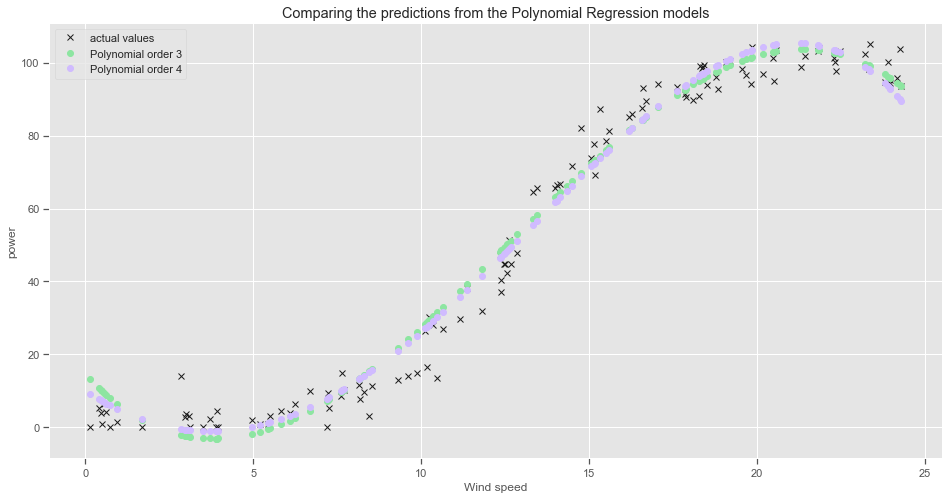
Plot the predictions from the Polynomial Regression Models:
### Plot the predictions from the models
plt.rcParams['figure.figsize'] = (16, 8)
plt.style.use('seaborn-colorblind')
plt.plot(X_test, y_test, 'kx',label ='actual values')

plt.plot(X_test, poly3_predictions, 'go', label="Polynomial order 3")
plt.plot(X_test, poly4_predictions, 'mo', label="Polynomial order 4")
plt.xlabel("Wind speed")
plt.ylabel("power")
plt.title("Comparing the predictions from the Polynomial Regression models")
plt.legend()
plt.savefig("images/Comparing the predictions from the Polynomial Regression models")
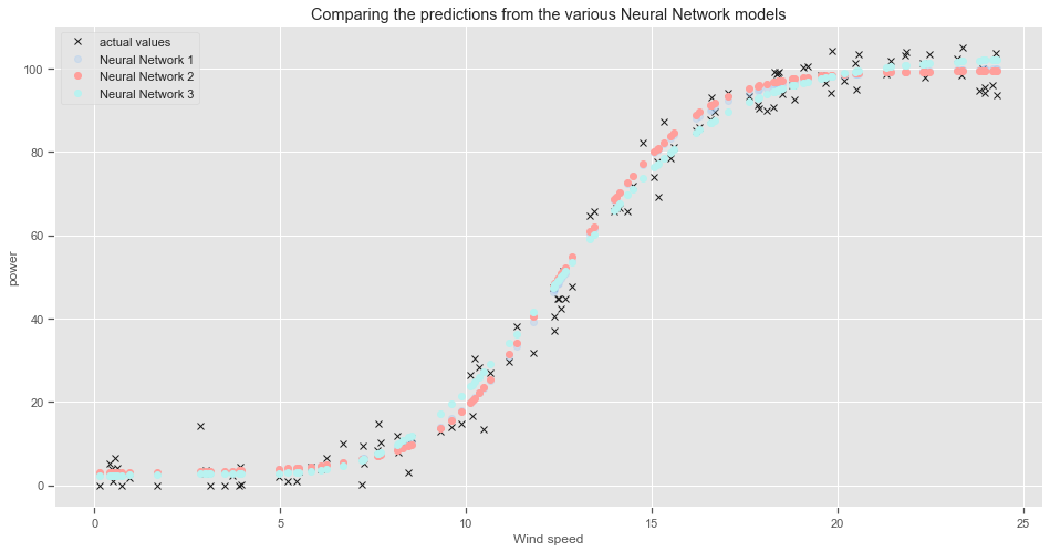
Plot the predictions from the Neural Network Models:
### Plot the predictions from the models
plt.style.use('seaborn-colorblind')
plt.plot(X_test, y_test, 'kx',label ='actual values')

plt.plot(X_test, model_predictions,'bo', alpha=0.3,label="Neural Network 1")
plt.plot(X_test, model2_predictions, 'ro', label="Neural Network 2")
plt.plot(X_test, model3_predictions, 'co', label="Neural Network 3")

plt.xlabel("Wind speed")
plt.ylabel("power")
plt.title("Comparing the predictions from the various Neural Network models")
plt.legend()
plt.savefig("images/Comparing the predictions from the various Neural Network models")
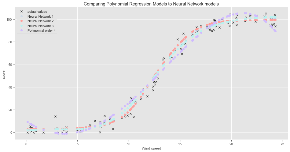
Plot the predictions from the Polynomial Regression models vs the Neural Network Models:
### Plot the predictions from the models
plt.style.use('seaborn-colorblind')
plt.plot(X_test, y_test, 'kx',label ='actual values')

plt.plot(X_test, model_predictions,'bo', alpha=0.3,label="Neural Network 1")
plt.plot(X_test, model2_predictions, 'ro', label="Neural Network 2")
plt.plot(X_test, model3_predictions, 'co', label="Neural Network 3")
plt.plot(X_test, poly4_predictions, 'mo', label="Polynomial order 4")

plt.xlabel("Wind speed")
plt.ylabel("power")
plt.title("Comparing Polynomial Regression Models to Neural Network models")
plt.legend()
plt.savefig("images/Comparing Polynomial Regression Models to Neural Network models")
There is not much difference between the 3rd and 4th order polynomial regression models. The 4th degree polynomial regression model does not go as far into negative power values. Both regression lines tend to over estimate the power output for wind speed values in the range between 8 and 15 metres per second approximately, then underestimate the power output values for higher wind speed values.
The ideal loss is is zero and the ideal accuracy is 1.0 or 100%.
Look at evaluation metrics for the two types of models:
While the regression models performed pretty well overall given its relative simplicity, the neural networks had a lower overall cost. There is a higher computational cost involved though and it does take more time to run.
Polynomial Regression models:
print("Evaluating the polynomial regression model with 3 degrees:")
print('Mean squared error: %.2f' % mean_squared_error(y_test,poly3_predictions ))
# The coefficient of determination: 1 is perfect prediction
print('Coefficient of determination: %.2f' % r2_score(y_test, poly3_predictions))
print('Root Mean Squared Error: %.2f' % np.sqrt(mean_squared_error(y_test,poly3_predictions )))
Evaluating the polynomial regression model with 3 degrees:
Mean squared error: 33.32
Coefficient of determination: 0.98
Root Mean Squared Error: 5.77
print("Evaluating the polynomial regression model with 4 degrees:")
print('Mean squared error: %.2f' % mean_squared_error(y_test,poly4_predictions ))
# The coefficient of determination: 1 is perfect prediction
print('Coefficient of determination: %.2f' % r2_score(y_test, poly4_predictions))
print('Root Mean Squared Error: %.2f' % np.sqrt(mean_squared_error(y_test,poly4_predictions )))
Evaluating the polynomial regression model with 4 degrees:
Mean squared error: 30.80
Coefficient of determination: 0.98
Root Mean Squared Error: 5.55
print("RMSE from Neural Network 1")
print('Training data RMSE: %.3f, Test data RMSE: %.3f' % (train_rmse, test_rmse))
print("\nRMSE from Neural Network 2")
print('Training data RMSE: %.3f, Test data RMSE: %.3f' % (train_rmse2, test_rmse2))
print("\nRMSE from Neural Network 3")
print('Training data RMSE: %.3f, Test data RMSE: %.3f' % (train_rmse3, test_rmse3))
RMSE from Neural Network 1
Training data RMSE: 4.093, Test data RMSE: 4.127

RMSE from Neural Network 2
Training data RMSE: 4.101, Test data RMSE: 4.305

RMSE from Neural Network 3
Training data RMSE: 4.419, Test data RMSE: 4.338
#import tensorflow.keras as kr
#from tensorflow.keras.models import load_model
#model = load_model('model.h5')
#model2=load_model('model2.h5')
#import pickle
#import joblib
# In the specific case of scikit-learn, it may be better to use joblib’s replacement of pickle
#from joblib import dump, load

#model_poly3 = joblib.load('model_poly3.joblib')
#mod_poly3 = joblib.load('model_poly3.pkl')
#mod_poly4 = joblib.load('model_poly4.joblib')