Machine Learning and Statistics Project 2020

This notebook forms part of the requirement for the Machine Learning and Statistics project 2020 submitted as part of the Higher Diploma in Computing and Data Anaytics at GMIT by Angela Carpenter.

Project Instructions

The aim of this project is to create a web service that uses machine learning to make predictions based on the data set powerproduction available on Moodle. The goal is to produce a model that accurately predicts wind turbine power output from wind speed values, as in the data set. A web service must also be developed that will respond with predicted power values based on speed values sent as HTTP requests.

In this notebook I trained and developed machine learning models using the data set. The models used are explained and the accuracy of the models are analysed. The models used are polynomial regression models and artificial neural networks.

  • The first section of the notebook get the data and performs some exploratory data analysis on it.
  • The next section provides some background on power output from wind turbines for some context and to understand the data involved.
  • The machine learning models used are explained in the next section before applying each model to the data and evaluating the performance and the accuracy of the models.
  • The machine learning models used are then compared to each other to determine which model more accurately predicts power output based on the wind speed values in this dataset.
  • References are listed at the end of the notebook.

Importing Python libraries:

In [1]:
# first importing the following libraries
import numpy as np
# pandas dataframes
import pandas as pd  
# plotting library
import matplotlib.pyplot as plt 
# another plotting library
import seaborn as sns
# splitting dataset into training and testing sets
import sklearn
print(sklearn.__version__)
from sklearn.model_selection import train_test_split
# for polynomial regression 
from sklearn.preprocessing import PolynomialFeatures
# for linear regression 
from sklearn.linear_model import LinearRegression
from sklearn import linear_model
# for evaluation metrics
from sklearn.metrics import mean_squared_error, r2_score
# neural networks
import tensorflow.keras as kr
from tensorflow.keras import Sequential
from tensorflow.keras.layers import Dense
# save a model in scikit-learn by using Python’s built-in persistence model pickle:
import pickle
# In the specific case of scikit-learn, it may be better to use joblib’s replacement of pickle
import joblib
from joblib import dump, load
print (joblib.__version__)
0.23.2
0.16.0

Importing the dataset:

The dataset is available from Github.[1]

In [2]:
# save link to data and reference the link 
csv_url = 'https://raw.githubusercontent.com/ianmcloughlin/2020A-machstat-project/master/dataset/powerproduction.csv'
# read the csv data into a pandas dataframe
df = pd.read_csv(csv_url)
df
# write the dataframe to csv
df.to_csv('df.csv')
# make a copy of the dataframe
dfx = df.copy()

Exploratory Data Analysis on the dataset:

The power variable represents wind turbine power output and the speed values are wind speed values. This is all that has been provided. There are no null values in the dataset but there are 49 observations with zero values. While there is only one zero value for the speed variable, there are 49 zero values for the power variable. Some research below suggests that the wind speed values are measured in metres per second and that the power values are measured in kilowatts, although it could be megawatts based on the values in the dataset. However this will not affect the analysis.

Exploratory data analysis generally involves both non-graphical methods which include calculation of summary statistics and graphical methods which summarises the data in a picture or a plot. Visualisations can highlight any obvious relationships between the different variables in the dataset and to identify any groups of observations that are clearly separate to other groups of observations.

In [3]:
df.head()
Out[3]:
speed power
0 0.000 0.0
1 0.125 0.0
2 0.150 0.0
3 0.225 0.0
4 0.275 0.0
In [4]:
df.tail()
Out[4]:
speed power
495 24.775 0.0
496 24.850 0.0
497 24.875 0.0
498 24.950 0.0
499 25.000 0.0
In [5]:
#  have a look at the dataset
df.sort_values(by='power', ascending=False).head()
df.sort_values(by='power').head()
df.sort_values(by='speed').head()
# check for null values
df.isnull().values.any()
df.isnull().sum()
# check for zero values
df.isin([0]).sum()
Out[5]:
speed     1
power    49
dtype: int64

Looking at the distribution of the data:

A histogram can be used to show the distribution of a single quantitative variable such as speed or power values, including the centre and spread of the distribution and if there is any skew in the data. Wind speed appears to be uniformly distributed with values spread out from zero up to a maximum value of 25. Power output values on the other hand looks to be bimodal with two defined peaks, one around zero power values and the second around the 100 kilowatt mark. The first peak is betweeen power values of 0 and 5. This is not surprising given the large number of zero power values in this dataset. Almost 10% of the power values supplied are zero. There is another smaller peak around values of 95-100. Most of the remaining power values fall between 18 and 85.

In [6]:
    %matplotlib inline

    # plot the histograms of Speed values
    f, axs = plt.subplots(1, 2, figsize=(12, 5))
    sns.histplot(data=df, x="speed", ax=axs[0], bins=20, kde=True,color="blue")
    sns.histplot(data=df, x="power", alpha=.8, legend=False, ax=axs[1], bins=20, kde=True, color="purple")

    #plt.title("Speed vs Power");
    plt.suptitle("The Distribution of the Wind Speed and Power Output variables")
    plt.savefig("images/The Distribution of the Wind Speed and Power output variables.png")
    f.tight_layout()

The relationship between the Wind Speed and Power Output variables:

In [7]:
# create the plot
plt.style.use('ggplot')
# Plot size.
plt.rcParams['figure.figsize'] = (14, 8)


plt.scatter(df['speed'],df['power'], marker=".")
# https://stackoverflow.com/questions/12608788/changing-the-tick-frequency-on-x-or-y-axis-in-matplotlib
plt.yticks(np.arange(min(df['power']), max(df['power'])+1, 5.0))
plt.xticks(np.arange(min(df['speed']), max(df['speed'])+1, 2.0))
#sns.scatterplot(x=df['speed'],y=df['power'], marker="x")
plt.grid(True)
plt.xlabel("Wind speed (m/s)")
plt.ylabel("Power (kilowatts)")
# add title
plt.title("Wind Speed vs Power Output", fontsize=20);
plt.savefig("images/Wind Speed Power scatterplot.png")
plt.show()

Scatter plots are useful to identify trends and patterns in a dataset which might indicate a relationship between two numerical variables such as we have in this dataset. The ordered pairs of numbers consisting of the independent variable wind 'speed' and the dependent variable 'power' output are plotted below resulting in a joint distribution of the two variables. Each point represents an actual observation is the dataset with a speed and a corresponding power value. The scatter plot above shows an increasing linear trend in the middle range of the wind speed values. This would indicate that for increasing wind speeds in this range, power output values do increase, but only after a minimum wind speed has been reached. Power outputs then increase in line with increases in wind speed until it reaches a peak and levels off. The plot suggests that very low winds may not be enough to get the turbine going and that the turbines have a maximum power level. Once the turbine is in motion perhaps little is required to keep it going. Some of the power generated might be consumed by the turbine itself at low levels to get it started.

Correlation and Covariance of Wind Speed and Power Output values:

For two quantitative variables such as the wind speed and power values, the covariance and correlation can also be used to determine whether a linear relationship between variables does exist and to show if one variable tends to occur with large or small values of another variable. The correlation statistics puts a numerical value on the strength and direction of the relationship. The correlation coefficient here of 0.85 shows there is a very strong positive relationship between the wind speed and turbine power output. The scatter plot shows a curved relationship between the variables. There appears to be a curvilinear pattern in the data.

In [8]:
df.corr()
Out[8]:
speed power
speed 1.000000 0.853778
power 0.853778 1.000000

Some summary statistics of the dataset:

When looking at quantitative variables such as wind speed and power values, the characteristics of interest are the centre, spread, modality, the shape of the distribution and the outliers. The central tendency or location of the data distribution is determined by the typical or middle values. While the mean value is the average value in the dataset it may not be typical of the values in the dataset if there are very small or very large values in the dataset. The median is another measure of central tendancy - it is the middle value after all the values are put in an ordered list. The mean and median are similar for symmetric distributions whereas for unimodal skewed distributions the mean will be more in the direction of the long tail of the distribution. The median can be considered a more typical value in the dataset or closer to some of the typical values and is also considered robust which means that removing some of the data will not tend to change the value of the median. A few extreme values will not affect the median as they would affect the mean. In this dataset the mean and median wind speed values are similar at approx 12.5 to 12.6 metres per second. The median power value is just over 41 unit compared to the mean power value of 48 (kws). As we saw above, there are many zero values for power in the dataset. At least 10% of the power values in the dataset are zero.

The variance and standard deviation statistics can be used to show the spread of the distribution of the speed and power data values and how far away from the centre the data points are located. The variance is the average of the squared deviations of each observation from the centre or mean of the data while the standard deviation is the square root of the variance and is in the same units as the data and therefore can be more easily interpreted. The range of values in the data is shown by the minimum and maximum values and is not considered a robust measure of spread but it is useful for showing possible errors or outliers.

The percentiles or quartiles of the speed and power values can be used to see the spread of the data values. The Interquartile range (IQR) is calculated by taking the 75% percentile or 3rd quartile minus the 25% percentile or first quartile and captures half of the values, the middle values of the data. Data that is more spread out will have a higher IQR. The IQR is considered a more robust measure of spread than the variance and standard deviation and will be more clearly shown in the boxplots further down. The IQR does not consider the data below the 25% percentile or above the 75% percentile which may contain outliers. The statistics here show that the power output variable in this dataset is much more spread out or variable than the wind speed variable.

In [9]:
# using pandas summary statistics of the numerical values
df.describe() 
Out[9]:
speed power
count 500.000000 500.000000
mean 12.590398 48.014584
std 7.224991 41.614572
min 0.000000 0.000000
25% 6.324750 5.288000
50% 12.550500 41.645500
75% 18.775250 93.537000
max 25.000000 113.556000
In [10]:
print("The mean speed value is %.3f" %df['speed'].mean(),"while the median speed value  is %.3f" %df['speed'].quantile(q=0.5))
print("The mean power value is %.3f" %df['power'].mean(),"while the median power value  is %.3f" %df['power'].quantile(q=0.5))
#print(f"The variance and standard deviations of speed values  are {df['speed'].var():.3f} and {df['speed'].std():.3f}")
#print(f"The variance and standard deviations of power values are {df['power'].var():.3f} and {df['power'].std():.3f}")
print(f"The standard deviations of speed values  is {df['speed'].std():.3f}")
print(f"The standard deviations of power values is {df['power'].std():.3f}")
print(f"The minimum speed value is {df['speed'].min()} while the maximum speed value is { df['speed'].max()} giving range of {df['speed'].max() - df['speed'].min()}")
print(f"The minimum Power value is {df['power'].min()} while the maximum power value is { df['power'].max()} giving range of {df['power'].max() - df['power'].min()}")
print(f"The median speed value is {df['speed'].quantile(q=0.5)} with the IQR ranging from {df['speed'].quantile(q=0.25):.2f} to  {df['speed'].quantile(q=0.75):.2f}")
print(f"The median power value is {df['power'].quantile(q=0.5)} with the IQR ranging from {df['power'].quantile(q=0.25):.2f} to  {df['power'].quantile(q=0.75):.2f}")
The mean speed value is 12.590 while the median speed value  is 12.550
The mean power value is 48.015 while the median power value  is 41.645
The standard deviations of speed values  is 7.225
The standard deviations of power values is 41.615
The minimum speed value is 0.0 while the maximum speed value is 25.0 giving range of 25.0
The minimum Power value is 0.0 while the maximum power value is 113.556 giving range of 113.556
The median speed value is 12.5505 with the IQR ranging from 6.32 to  18.78
The median power value is 41.6455 with the IQR ranging from 5.29 to  93.54
In [11]:
f, axes = plt.subplots(1, 2, figsize=(12, 4))
sns.set(style="ticks", palette="pastel")
sns.boxplot(y=df['speed'], ax=axes[0], color="blue")
# add a title
axes[0].set_title("Boxplot of Wind Speed values")
sns.boxplot(y=df['power'], ax=axes[1], color="purple")
axes[1].set_title("Boxplot of Power Output Values");
plt.savefig("images/Boxplots of Wind Speed and Power Output values.png")

The skewness of the data is a measure of assymetry which can be seen by the lopsidedness of a boxplot. Wind speed appears to be quite symmetric. The wind speed boxplot is cut pretty much in half by the median. Power appears to be somewhat skewed to the right as the boxplot shows more of the box to the right or above the median line. A boxplot with the median closer to the lower quartile is considered positively skewed. Positively skewed data has the mean greater than the median and it can be interpreted as having a higher frequency of high valued scores. The lower values of power are closer together than the higher power values.

Regression plots:

The Python Seaborn library has some regression plots that can be used to quickly visualise relationships and patterns that may exist in the data. They use statistical models to estimate a simple relationship between sets of observations and are mainly used to visualise patterns in a dataset during the exploratory data analysis. The scatter plot earlier showed a relationship between wind speeds and wind turbine power that is non-linear. There does seem to be a somewhat linear relationship for wind speeds between values of about 10 up to about 18 or so. The plot below shows that the polynomial with order 3 looks a much better fit to the line than the first or second order linear regression lines. It is important not to go down the road of overfitting the data though.

In [12]:
f, axes = plt.subplots(2, 2, figsize=(18, 8))
x = "speed"
y = "power"
sns.regplot(x="speed", y="power", data=df, ax=axes[0,0], label="order = 1", ci=False); axes[0,0].legend()
sns.regplot(x="speed", y="power", data=df, order=2, ax=axes[0,1], label="order =2", ci=False); axes[0,1].legend()
sns.regplot(x="speed", y="power", data=df, order=3, ax=axes[1,0], label="order =3", ci=False); axes[1,0].legend()
sns.regplot(x="speed", y="power", data=df, order=4, ax=axes[1,1], label = "order=4", ci=False); axes[1,1].legend()
plt.legend()
plt.suptitle("Trying higher order polynomial regression functions to Speed and Power values")
plt.savefig("images/Higher Order regression plots.png")

Residual plots can be used to check whether the simple regression model of speed ~ power is appropriate for a dataset. The seaborn residplot fits and removes a simple linear regression and then plots the residual values for each observation. Ideally, these values should be randomly scattered around y = 0. If there is structure in the residuals, this suggests that simple linear regression is not appropriate for the data. The residual plot here has a shape which suggest non-linearity in the data set as expected.

In [13]:
plt.rcParams['figure.figsize'] = (12, 5)
sns.residplot(x="speed", y="power", data=df, scatter_kws={"s": 80})
plt.title("Residual plot"); 
plt.savefig("images/Residual plot.png")

Some background on Wind Turbines power output.

The dataset [1] consists of two columns each containing 500 floating numbers under the column names speed and power. There are no other features provided. Therefore before I go any further I do a little research into the dataset which may help in understanding and interpreting the relationship between wind speed and power output from a turbine and also in determining what conclusions can be reached based on the dataset alone. The research below also highlights the limitations and uncertainty in predicting power generated from wind turbines using local wind speed data.

Some background to the project was provided in a lecture. In the electricity supply market, the producers usually sell their electricity ahead of time and enter a contract where they agree to produce a certain number of kilowatts of electricity during a particular time frame. The price is negotiated in advance of generating electricity and pushing it onto the supply grid. Wind farms supply electricity to the supply grid and negotiate prices in advance. It is more difficult for wind farms to predict exactly how much electricity they can generate at a future date compared to other electricity producers as their generation of electricity depends on wind power. For this reason predictions can be estimated based on meterological data from a weather prediction agent such as Met Eireann. The aim is to be able to predict that when wind speed is a certain amount that the power produced from the turbines is a certain amount.

The Irish Wind Energy Association (IWEA)[2] is the representative body for the Irish wind industry, working to promote wind energy as an essential, economical and environmentally friendly part of the country’s low-carbon energy future. They note here that in 2018 wind energy provided 29 per cent of Ireland’s electricity. Each quarter, both EirGrid and ESBN publish updated wind farm statistics for Ireland at ESBN Connected Wind Farms. There is currently 4,130 MW of installed capacity in the Republic of Ireland. The amount of electricity a turbine can generate depends on the type of turbine and the wind conditions at any time. There are many different models of turbines that can generate different amounts of electricity. Ireland’s largest wind farm is the Galway Wind Park in Connemara which has 3 MW turbines. Eirgrid's Smart grid dashboard[3] shows actual and forecast wind generation by day, week and month for all wind farms on the system while WindEurope[4] has some facts and issues about wind energy in Europe, in particular the section on Wind Energy Basics. Wind is caused by three things, the heating of the atmosphere by the sun, the rotation of the Earth and the Earth's surface irregularities:

Air under high pressure moves toward areas of low pressure – and the greater the difference in pressure, the faster the air flows and the stronger the wind! [4]

Energy is the ability to do work and can be categorised into either kinetic energy (the energy of moving objects) or potential energy (energy that is stored). Wind turbines take the kinetic energy that’s in the wind and convert that kinetic energy into mechanical power which is mostly used in the form of electricity. Wind energy captures the energy of the wind and converts it to electricity and is an alternative to burning fossil fuels. It comes from a natural and renewable resourse and it is clean as it produces no greenhouse gas, emits no air pollutants and uses very little water. A wind turbine is a device that converts kinetic energy from the wind into electricity. Their output ranges from as small as 100 kilowatts to as big as 12 megawatts. This suggests that the power values in the dataset for this project is not in kilowatts but possibly megawatts or may represent a wind farm rather than a single turbine. However this is of no consequence to this project.

According to the https://windeurope.org website [4], there are three main variables determining how much electricity a turbine can produce: wind speed, blade radius and air density. Stronger winds allow more electricity to be produced with higher turbines being more receptive to strong winds. We only have the values for wind speed in the dataset here so will have to assume that the other variables are constant. Wind turbines generate electricity at wind speeds of 4 – 25 metres per second. [4] The same article also outlines what happens when the wind doesn't blow. A wind farms location is usually chosen purposely and therefore when a wind turbine is not turning it is usually because of maintenance, or because it must be stopped for safety reasons in the case of strong winds or a storm. This should help account for the zero values we see in the dataset. The article does note that while sometimes there might not be enough wind to turn a turbine, the wind energy is not lost as the wind energy can be stored in energy storage systems for later use whenever wind levels are low. This may somewhat complicate the predictions from any machine learning models. The scatter plot above does show power values corresponding to wind speed values below 4 metres per second, with a few of these in the 10 to 15 power value range.

Another article looks at how to calculate power output of wind [5] and notes that most U.S. manufacturers rate their turbines by the amount of power they can safely produce at a particular wind speed, usually chosen between 24 mph or 10.5 m/s and 36 mph or 16 m/s. A formula illustrates the factors important to the performance of a wind turbine and notes that the wind speed V has an exponent of 3 applied to it meaning that even small increases in wind speeds result in a large increase in power. $Power=k.Cp \frac{1}{2}\rho AV^3$ where P = power output in kilowatts, Cp = Maximum power coefficient, $\rho$ is Air density, A = Rotor swept area, V = wind speed in mph, k = 0.000133 a constant to yield power in kilowatts. There are other more complex formulas mentioned in other articles but this is not relevent to this project. Additionally the article notes that although the calculation of wind power illustrates important features about wind turbines, the best measure of wind turbine performance is annual energy output. The difference between power and energy is that power (kilowatts kW) is the rate at which electricity is consumed, while energy (kilowatt-hours kWh) is the quantity consumed.

I came across a blog post [6] that use a linear equation to calculate ideal wind production, where the author notes that modeling results can be enhanced via statistical analysis of hyper-local time series such as meteorological data and energy production data. Each wind turbine manufacturer provides an ideal energy production curve for their turbines. The article provides a brief overview which is taken from another research article [7]. Of particular relevance is that a typical wind turbine has three main characteristic speeds, the cut-in speeds (Vc), rated speeds (Vr) and cut-out (Vs) speeds which explain the s-shaped curve we see for this dataset.

  • The turbine starts generating power when the wind speed reaches the cut-in value.
  • The rated speed is the wind speed at which the generator is producing the machine’s rated power.
  • The power generation is shut down to prevent defects and damage when the wind speed reaches the cut-out speed. It also mentions the differences between the ideal power curves which just describe the potentially maximum output versus reality taking into account many factors as well as measurement variations. In practice, however, wind turbines are never used under ideal conditions, and the empirical power curves could be substantially different from the theoretical ones due to the location of the turbine, air density, wind velocity distribution, wind direction, mechanical and control issues, as well as uncertainties in measurements. [7]

While the ideal power curves simply describe potentially maximum output, accuracy could be improved by using more accurate accurate weather forecasts or various statistical methods such as machine learning. We do not have historical data which we could use for statistical improvements but nor do we have hyper-local forecasts as we don't know the source or time frame of this particular dataset. Another article notes that real wind turbines do not achieve their theoretical limit as their performance is a function to of aerodynamics and the need to limit power capture once the rated generator power is reached, at ‘rated’ windspeed. The generator power, turbine diameter and bladeshape are optimized based on site characteristics such as annual average wind speed and the wind speed distribution. [8]

Turbine manufacturers measure their turbine’s ‘powercurve’ (the relationship between power output and windspeed) at turbine test sites where it is calculated from 10 minute averaged wind speed ($U=\bar{\mu}$) and power. The typical power curves have an s-shape where at wind speeds less than rated the energy capture is approximately proportional to $U^3$ (known as Region II). At wind speeds above rated, the bladepitch and generator torque are actively controlled to limit the power to the generator’s rated power (Region III). [8]

Variations in atmospheric conditions can lead to changes in turbine power output of 10% or more at the same wind speed. Turbulence and shear and not usually used in the power curves as they are considered difficult to include in turbine power predictions. The article also mentions that because of intermittency in the wind, wind turbines typically produce 20%–40% of their maximum possible output over the course of a year. They note that there is a lot of uncertainty in predicting power generation from a turbine using local wind speed data. If the amount of energy is overestimated then the site might not be as profitable as expected while underestimating the energy available at a site might lead to a site not being developed at all. This study also simulated the aerodynamic forces on the turbines blades and structures using an aerostructuraland simulator and created 1796 10-minute wind fields from a stochastic turbulence simulator. The data from the wind fields from the simulations were used to form a database of 1796 observations of 10-min average power (the response) as a function of wind speed, turbulence intensity, and shear exponent (the forcing). The researchers binned the power data into 1 m s$^{-1}$ wide bins and included a plot (figure 3 in the article) of the power curve which shows a Region II between 0.3 metres per second and about 11.5 metres per second, region III is from end the end of region II up to 25 which correspond exactly with our dataset.

Source: Figure 3. Power curve and operating regions for the WindPACT 1.5 MW turbine [8]

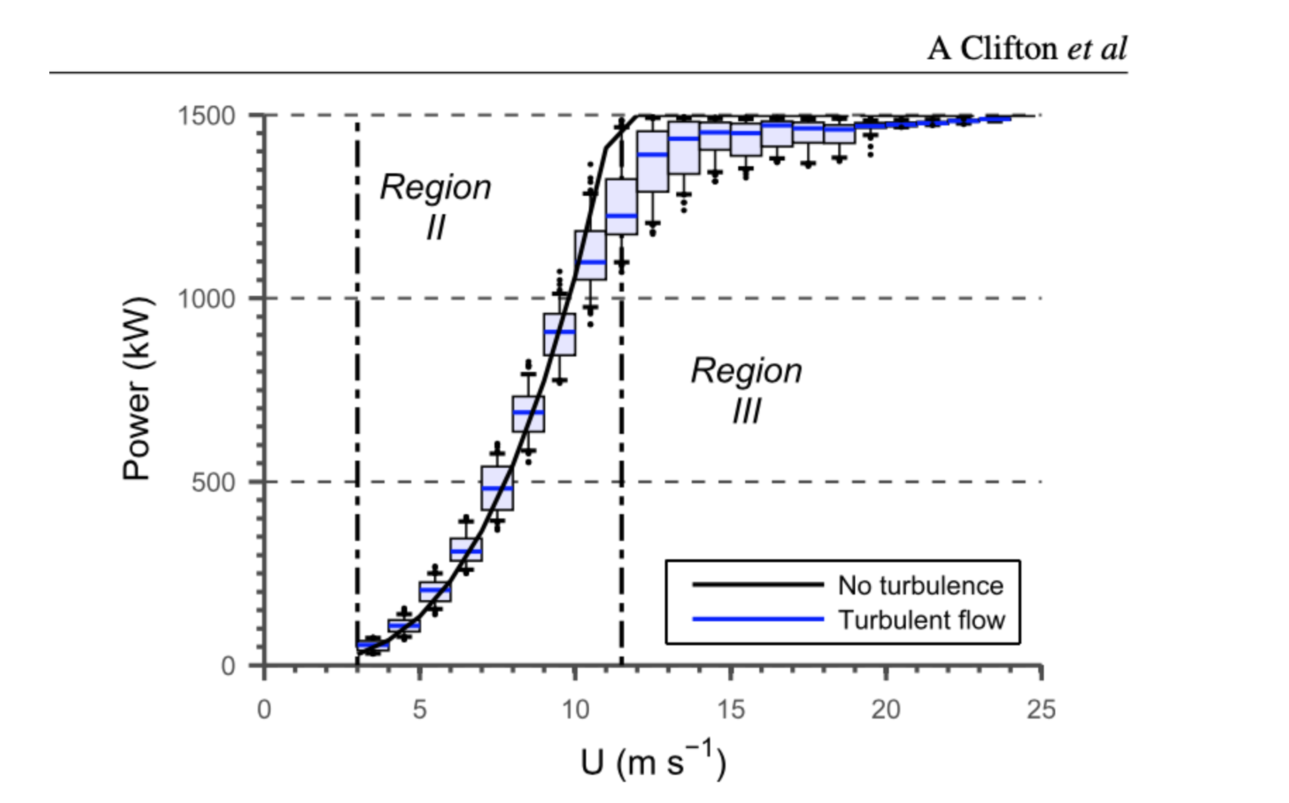
The authors also noted that although the forcing variables are evenly distributed, variance in power is largest near rated wind speed. This sensitivity may result in large variation between predicted power output and observed power output. Furthermore, the mean power generated in simulations that include turbulence is lower than the no-turbulence cases near rated wind speed. At wind speeds below 8 m s$^{-1}$, power increases with turbulence intensity and shear. The increase in power due to turbulence arises because turbulent flow with mean speed U carries more power than laminar flow of the same U. The changes in power output of +/-20% associated with turbulence are approximately half of the change due to a change in wind speed from 7 to 8 m s$^{−1}$. In contrast, at wind speeds just above and below rated speed, increasing turbulence intensity reduces power output as the turbine cannot capture the extra energy that gusts bring, but a short duration slow down to wind speeds below rated results in a loss of energy. As the mean wind speed increases, the total amount of time with the blades pitched toward feather increases and the wind turbine is more often operating at rated power. At wind speeds much greater than rated, larger turbulence intensities are required to reduce the output of the machine to less than rated power, regardless of shear.

The same article next looked at using machine learning to predict power output under different conditions by incorporating turbulence intensity and wind shear into power prediction tools. They note that the power output from the turbine is not a linear function of wind speed and so linear regression is not an appropriate technique. Non-linear regression assumes that the relationships are constant throughout the model space (i.e. power output is always proportional to $U^n$ ), which is incorrect, so non-linear regression is also inappropriate. Also, as multivariate bins only work where the training data includes data in all bins this would be computationally or observationally more expensive. Instead they chose a machine learning technique regression trees for capturing non-linear changes in response to forcing. Regression trees are models that use simple branching question paths to predict an outcome based on inputs. I don't think this is really an option for this project though as this particular dataset has only a single feature.

The turbines responds differently to changes in shear and turbulence at different wind speeds. In Region II, at wind speeds below 8 m s$^{−1}$, power output increases by up to 10% as turbulence increases or as the magnitude of the shear increases. At wind speeds greater than 8 m s$^{−1}$ and in Region III, the regression tree modeled power is consistent with the simulated power output: power decreases as turbulence intensity increases and shows weak or no dependence on shear.

The article concludes:

simulations suggest and the model clearly demonstrates that the response of the turbine is a complex non-linear function of hub height wind speed, turbulence intensity, and rotor disk shear. At wind speeds below rated speed, the turbine power output is most sensitive to changes in wind speed and speed, turbulence. At rated speed, the turbine is most sensitive to turbulence intensity and shear, and power can change by 10% under typical atmospheric conditions. At wind speeds greater than rated, the turbine responds most to changes in turbulence intensity.

The article also includes a figure of the power curves for different utility-scale wind turbines which all reach higher maximum powers than the values in this dataset. [8] The cut-in speeds quoted here are in miles per hour which can be converted to metres per second by divide by 2.237. Rated windspeed is the wind speed at which a turbine hits its maximum rated power output.

Wikipedia describes wind turbine design as follows:

A wind turbine is designed to produce power over a range of wind speeds. The cut-in speed is around 3–4 m/s for most turbines, and cut-out at 25 m/s. If the rated wind speed is exceeded the power has to be limited. There are various ways to achieve this. All wind turbines are designed for a maximum wind speed, called the survival speed, above which they will be damaged. The survival speed of commercial wind turbines is in the range of 40 m/s (144 km/h, 89 MPH) to 72 m/s (259 km/h, 161 MPH). The most common survival speed is 60 m/s (216 km/h, 134 MPH). Some have been designed to survive 80 metres per second (290 km/h; 180 mph) [9]

Every wind turbine design has a cut-in wind speed, a rated wind speed, and a cut-out wind speed. At the cut-in wind speed, the blades start to turn and a trickle of electricity starts to be produced. Around cut-in, the generator may be used as a motor to help the wind overcome inertia and start the blades turning.[10] The cut-in speed is typically 7 to 9 mph or equivalently to 3 to 4 meters per second. At the rated wind speed, the turbine is able to generate electricity at its maximum, or rated, capacity. The rated speed is usually in the range of 25 to 35 mph (equivalent to 11 to 13.5 metres per second). At the cut-out wind speed, the turbine shuts down to avoid damage. The pitch controllers feather the blades to let the wind flow past them and the rotor hub is braked. The wind usually has to return to a much lower speed, called the cut-back-in wind speed, for a certain amount of time before the turbine will restart. The cut-out speed is generally around 55 mph (24.6 metres per second). The cut-back-in speed is around 45 mph (20 metres per second).[10]

Some notable facts from this research that may be of relevance to this project:

  • Wind speed is measured in metres per second. (The actual metrics are not provided in the dataset)
  • Wind turbines generate electricity at wind speeds of 4 – 25 metres per second [4]
  • A wind farms location is usually chosen purposely and therefore when a wind turbine is not turning it is usually because of maintenance, or because it must be stopped for safety reasons in the case of strong winds or a storm. This would account for the zero values in the dataset.
  • Sometimes there might not be enough wind to turn a turbine but the wind energy is not lost as it can be stored up to be used later whenever wind levels are low. This might explain the higher than expected values of power for low levels of wind speed that we see in the dataset.
  • Turbines are rated by the amount of power they can safely produce at a particular wind speed, usually chosen between 24 mph or 10.5 m/s and 36 mph or 16 m/s [5].
  • In formulas used to illustrate the factors important to the performance of a wind turbine, an exponent of 3 is applied to wind speed. Small increases in wind speeds result in a large increase in power. [5]
  • Of particular relevance is that a typical wind turbine has three main characteristic speeds, the cut-in speeds (Vc), rated speeds (Vr) and cut-out (Vs) speeds. This helps explain the s-shaped curve we see for this dataset [7]
    • The turbine starts generating power when the wind speed reaches the cut-in value.
    • The rated speed is the wind speed at which the generator is producing the machine’s rated power.
    • The power generation is shut down to prevent defects and damage when the wind speed reaches the cut-out speed.
  • There is a lot of uncertainty around the prediction of power generation from a turbine using local wind speed data.
  • Variance in power is largest near rated wind speed and this sensitivity may result in large variation between predicted power output and observed power output.

Back to the dataset:

The scatter plot of our dataset did show three distinct sections of the curve, the first section at low values of wind speed where the wind turbine values are clustered around zero (including the 10% of observations that have zero power values), the second section where there seems to be an increasing linear trend between wind speed and power output and thirdly the last section where the values of power have reached a peak at higher wind speeds and level off, and also the outliers here. We would expect to see power being generated when speed is above 3-4 metres per second. The scatter plot shows power output values below wind speeds of below this. The cut-out speed from the scatter plot and values is 24.4 metres per second. The cut back in speed after cut out is 20 meters per second. This might explain some of the variation in power values around this speed range in our dataset. There are no null values in the dataset but there are 49 datapoints where power value is zero representing 10% of the observations. There is a single data point where speed value is zero as well as power.

  • Ten speed values over 24.4 metres per hour with a corresponding power value of zero
  • There are no data points with speeds above 24.4 and power not equal to zero
  • Eight data points where speed is less than 8 metres per second and power value is zero
  • Four datapoints where speed is greater than 8 and less than 24.4 metres per second and corresponding power values are zero
  • 24 datapoints where speed is less than 4 metres per second and power is zero
  • The cut-in speed is typically 3 to 4 meters per second. There are 17 observations where speed is less than 3 metres per second.

Non-zero power values where speed is less than 3 metres per second:

There are 39 observations where speed is less than the cut-in speed (of between 3 and 4 metres per second) and the corresponding power value is greater than zero. I think these will be the tricky ones to predict. There was mention in an article referenced above [4] that while sometimes there might not be enough wind to turn a turbine, the wind energy is not lost as the wind energy can be stored in energy storage systems for later use whenever wind levels are low.

Rated speed

At the rated wind speed, the turbine is able to generate electricity at its maximum, or rated, capacity. The rated speed is usually in the range of 25 to 35 mph. (equivalent to 11.18 to 13.4 metres per second). This is based on the research above but we don't know the details of the actual wind turbines being used here. The rated speed for the turbines in this dataset must be greated than this range as they do not reach their maximum capacity until wind speed is greater than 15 metres per second. The max power value in the dataset is 113.556 kws but there are very few observations in the dataset where power is greater than 110. The power curve for this dataset shows the power values levelling off in and around values between 90 and 100.

Unique values in the dataset:

In [14]:
# show the unique values
df.speed.unique()
len(df.groupby('speed')) # 490
# a count of the unique speed values
df.speed.value_counts() # 490
# a count of the unique power values
df.power.value_counts() # 451
df.groupby('speed')['power'].agg(['count', 'size', 'nunique'])
len(df.groupby('power')) # 451

df.groupby('power')['speed'].agg(['count', 'size', 'nunique'])
len(df[['speed', 'power']].drop_duplicates()) # 490
# the rows where both values are zero
df[(df['speed']==0) & (df['power']==0)].count() # only 1
df[df.power==0].count() # 49
Out[14]:
speed    49
power    49
dtype: int64

Number of zero wind speed values in the dataset:

In [15]:
print("The number of observations with a zero power value are as follows:")
print(f"For speed values below 3 metres per second: {df[(df.speed <3) & (df.power==0.0)].count()[0]}")
print(f"For speed values is between 3 and 4 metres per second: {df[(df.speed >3) & (df.speed <4) & (df.power==0.0)].count()[0]}")
print(f"For speed values between 4 and 7 metres per second: {df[(df.speed >4) & (df.speed<7) & (df.power==0.0)].count()[0]}")
print(f"For speed values between 7 and 24.4 metres per second: {df[(df.speed >7) & (df.speed<24.4) & (df.power==0.0)].count()[0]}")
print(f"For speed values above 24.4 metres per second: {df[(df.speed>24.4) & (df.power==0.0)].count()[0]}")
The number of observations with a zero power value are as follows:
For speed values below 3 metres per second: 17
For speed values is between 3 and 4 metres per second: 7
For speed values between 4 and 7 metres per second: 9
For speed values between 7 and 24.4 metres per second: 6
For speed values above 24.4 metres per second: 10
In [16]:
df[(df.speed < 3) & (df.power>0.0)].count() # 39
df[(df.speed < 3) & (df.power==0.0)].count() # 17
df[(df.speed < 4) & (df.power>0.0)].count() # 56
df[(df.speed < 4) & (df.power==0.0)].count() # 24
Out[16]:
speed    24
power    24
dtype: int64

Number of Power Output values greater than 100:

In [17]:
print(f"Number of data points where power is between 80 and 90 kws: {df[(df.power>80)&(df.power<90)].count()[0]}")
print(f"Number of data points where power is between 90 and 100 kws: {df[(df.power>90)&(df.power<100)].count()[0]}")
print(f"Number of data points where power is between 100 and 110 kws: {df[(df.power>100)&(df.power<110)].count()[0]}")
print(f"Number of data points where power is greater than 110 kws: {df[(df.power>110)].count()[0]}")
Number of data points where power is between 80 and 90 kws: 31
Number of data points where power is between 90 and 100 kws: 95
Number of data points where power is between 100 and 110 kws: 55
Number of data points where power is greater than 110 kws: 2

Cut-out speeds for safety reasons:

At the cut-out wind speed, the turbine shuts down to avoid damage. There are 10 observations that fall into the cut-out speed range. There are no datapoints at all where speed is above the cut-out speed value and power value is not zero.

In [18]:
# there are no points in the dataset where speed is greater than 24.4 and power value is not zero
print(f"Number of observations where speed values is above 24.4 metres per second: {df[df.speed>24.4].count()[0]}") # 
print(f"Number of observations where power values is zero and speed is above 24.4 metres per second: {df[(df.speed > 24.4) & (df.power==0.0)].count()[0]}")
Number of observations where speed values is above 24.4 metres per second: 10
Number of observations where power values is zero and speed is above 24.4 metres per second: 10

Speeds between 7 and 8 metres per second:

In [19]:
df[(df.speed >7) & (df.speed < 8) & (df.power==0.0)].count()
Out[19]:
speed    2
power    2
dtype: int64
In [20]:
df[(df.speed >11) & (df.speed< 13.4)].count()
Out[20]:
speed    49
power    49
dtype: int64

Data cleaning:

I debated whether to leave in the observations with zero power values as they do convey some information about the dataset. However after initially trying out the neural network using the complete dataset, the cost did not fall as much as desired and the resulting plots suggested that keeping the zero power values in for the very high values of speed were throwing things out. The research above showed that there is a cut-out speed between 24 and 25 metres per second for safety reasons. At the cut-out wind speed, the turbine shuts down to avoid damage. This is enough to justify excluding these observations as we can predict that the power output will be zero when the wind speed exceeds this cut out value. There are only ten observations in the dataset that fall into this range. We can only predict values for power when the turbines are turned on and therefore maybe the model should only be predicting for values of speed where the turbine is on!

While there is only one zero value for the speed variable, there are 49 zero values for the power variable. These mostly occur below a certain value of speed but located alongside non-zero power values and there are a few that are associated with medium and higher speed values of speed. Most of the data points in the dataset are unique values. The one datapoint with a zero speed value has a zero power value as expected.

Summary of where the zero power values occur:

  • 17 where speed is less than 3 metres per second
  • 7 where speed is between 3 and 4 metres per second. This is the cut-in speed
  • 9 where speed lies between 4 and 7
  • 6 where speed is between 7 and 24.4
  • 10 where speed is above 24.4 metres per second. This is the cut-out value.

Wind turbines generate electricity at wind speeds of 4 – 25 metres per second. For now I will drop all observations where speed is greater than the cut-out value of 24.4 metres per second. I will also drop the observations above the cut-in speed of between 3 and 4 metres per second. I will leave in all the observations where speed is less than the cut-in speed including the zero values. Therefore I am dropping 25 observations from the dataset where the power values are zero.

  • Ten observations where the wind speed is greater than the cut-off value; the corresponding power is zero as the turbines are off.
  • Fifteen observations where wind speed is greater than the cut-in and less than the cut-out and the power is zero.

I am assuming that these represent points where the turbines have been turned off for maintenance or other reasons. I may revisit this. I will make a copy of the dataframe for this purpose.

Excluding the zero values results in the models over predicting the power values for the higher values of speed. Leaving in the zero values does pull the curves back down but only after the max speed has been exceeded.

In [21]:
#https://pandas.pydata.org/pandas-docs/stable/reference/api/pandas.DataFrame.drop.html
# https://thispointer.com/python-pandas-how-to-drop-rows-in-dataframe-by-conditions-on-column-values/
#df.drop(df.loc[(df.speed>24.4)].index, inplace=True)
In [22]:
# make a copy of the dataframe
dfx = df.copy()
In [23]:
# how many rows where wind speed above the cut-in speed and power is zero
dfx.loc[(dfx.speed > 4)&(dfx.power == 0)].count()
Out[23]:
speed    25
power    25
dtype: int64
In [24]:
# drop rows from the new dataframe 
dfx.drop(dfx.loc[(df.speed > 4)&(dfx.power == 0)].index, inplace=True)
In [25]:
# summary statistics
dfx.describe()
Out[25]:
speed power
count 475.000000 475.000000
mean 12.440971 50.541667
std 7.101231 41.171815
min 0.000000 0.000000
25% 6.293500 6.737500
50% 12.538000 47.282000
75% 18.531500 94.017500
max 24.399000 113.556000

Machine Learning Model 1 - Polynomial Regression

The goal of the project is to predict wind power from wind speed and therefore this problem falls into supervised learning. Supervised machine learning is about creating models that precisely map the given inputs (independent variables, or predictors) to the given outputs (dependent variables, or responses).[11]

Regression involves predicting a continuous-valued attribute associated with an object. It is a statistical method used to describe the nature of the relationship between variables which could be positive or negative, linear or nonlinear. Scatter plots visualise a relationship and the correlation coefficient is a measure of the strength of a linear relationship. The correlation statistics show a high correlation between the variables with a value of 0.85. If a scatter plot and the value of the correlation coefficient indicate a linear relationship, the next step is to determine the equation of the regression line which is the data's line of best fit. Often one of the variables is fixed or controlled and is known as the independent or explanatory variable, the aim is to determine how another variable varies known as the dependent or response variable varies with it. The explanatory variable is usually represented by X while the dependent or response variable is represented by y. Least squares linear regression is a method for predicting the value of a dependent variable y such as power, based on the value of an independent variable x such as wind speeds.

Regression plots were shown above in the exploratory data analysis section, simple linear regression does not adequately model the relationship between the wind and speed values over the entire dataset as there are sections of the datasets that are either above or below the simple linear regression line. The higher order polynomials regression curves have more parameters and do seem to capture more of the relationship between wind speed and power output values. The fourth order polynomial does seem to be even better for the datapoints at the lower end of wind speed values. However it is important not to overfit the data either as then the model will not capture the general trend of the data. There was a suggestion in the research above that an exponent of 3 can be applied to the wind speed factor. [5]. The typical power curves have an s-shape where at wind speeds less than rated the energy capture is approximately proportional to $U^3$ [8] where ($U=\bar{\mu}$) is the 10 minute averaged wind speeds.

For my first machine learning model I will develop two polynomial regression model using the scikit-learn package.

One common pattern within machine learning is to use linear models trained on nonlinear functions of the data. This approach maintains the generally fast performance of linear methods, while allowing them to fit a much wider range of data. [12]

A simple linear regression can be extended by constructing polynomial features from the coefficients. A regression model that is used to model the expected value of a dependent variable y in terms of an independent variable x can be represented by the equation $y=ax+b$. Adding a squared term will create a quadratic model of the form $y=a+b1x+b2^2+e$ where a is the intercept and e is the error rate. Adding a cubed term can be represented by the equation $y=a+b1x+b2x^2+b3x^3+e$. Additional terms can be added. The regression function is linear in terms of the unknown variables and therefore the models are still considered linear from the point of estimation.[15] Scikit-learn's PolynomialFeatures transforms an input data matrix into a new data matrix of a given degree. Adding an $X^3$ allows us to check if there is a cubic relationship in the data. A polynomial is a special case pf a linear model that is used to fit non-linear data. Adding polynomials to the regression is like multiple linear regression, as you are adding extra variables in the form of powers of each feature as new features. [13]

Regression plots on the cleaned data:

Below are the regression plots using Seaborn regplot function with a 3rd and 4th order applied on the cleaned dataset that excludes some of the zero value observations.

In [26]:
f, axes = plt.subplots(1, 2, figsize=(14, 6))
x = "speed"
y = "power"

sns.regplot(x="speed", y="power", data=dfx, order=3, ax=axes[0], label="order =3", ci=False,marker="x", color="blue"); axes[0].legend()
sns.regplot(x="speed", y="power", data=dfx, order=4, ax=axes[1], label = "order=4",marker='x', color="green"); axes[1].legend()
plt.legend()
plt.suptitle("Polynomial regression functions applied to the data")
plt.savefig("images/Polynomial regression functions.png")

Split data into training and test sets

Splitting your dataset is essential for an unbiased evaluation of prediction performance. The dataset can be split into two or three random subsets.

  • A training set: used to train or fit your model. Training set are used to find the optimal weights or coefficients for linear regression, logistic regression, or neural networks.
  • A validation set: subset used for unbiased model evaluation during hyperparameter tuning. For each set of hyperparameters, fit the model with the training set and assess it's performance with the validation set.
  • A test set used for an unbiased evaluation of the final model. This should not be used for fitting or validating the model. In less complex cases, when you don’t have to tune hyperparameters, it’s okay to work with only the training and test sets. [11]

Splitting a dataset can also be used for detecting if your model suffers from problems such as underfitting and overfitting.

Underfitting usually arises when a model fails to capture the relationships among data. This can occur when you try to represent non-linear relationships with a linear model. Overfitting occurs when a model has an excessively complex structure and learns both the existing relationships between the variables as well as the noise. Overfitted models usually fail to recognise the general trend of the data. While underfitted models are likely to have poor performance with both the training and testing dataset, overfitted models will usually have strong performance on the training dataset but will have poor performance on the unseen test set. Scikit-learn has a module for splitting the data into training and test sets. The default split is 75% for the training set and 25% for the test set. The random state can be set to make the split reproducible. I initially did not use this but it makes it harder to compare the different machine learning models if you have a different training and test set for each.

Using scikit-learn to split the dataset into training and test subsets:

using sklearn.model_selection.train_test_split

In [27]:
# split into input and output columns

X, y = dfx.values[:, :-1], dfx.values[:, -1:]
# split into train and test datasets
X_train, X_test, y_train, y_test = train_test_split(X, y, test_size=0.25, random_state=0)
print(X_train.shape, X_test.shape, y_train.shape, y_test.shape)
# determine the number of input features

n_features = X_train.shape[1]
(356, 1) (119, 1) (356, 1) (119, 1)

Full dataset df:

To use the full dataset df including the zero power values change uncomment the line below

In [28]:
# split the dataset into input and output columns: df is the full dataset
#X, y = df.values[:, :-1], df.values[:, -1:]

Cleaned dataset dfx:

In [29]:
# split the dataset into input and output columns: dfx is the cleaned dataset
X, y = dfx.values[:, :-1], dfx.values[:, -1:]
In [30]:
# split into train and test datasets
X_train, X_test, y_train, y_test = train_test_split(X, y, test_size=0.25, random_state=0)
print(X_train.shape, X_test.shape, y_train.shape, y_test.shape)
# determine the number of input features
n_features = X_train.shape[1]
(356, 1) (119, 1) (356, 1) (119, 1)

Transform the features of x

Scikit-learns PolynomialFeatures can be used to add a cubic variable or a 4th degree variable to the dataset. Once transformed the new polynomial features can be used with any linear model. The two regression models are developed alongside each other for convenience.

In [31]:
# using scikit-learn, set the order to 3 degrees to include a cubic 
# include_bias=False otherwise I end up with a column of zeros 
poly3 = PolynomialFeatures(degree=3, include_bias=False)
poly4 = PolynomialFeatures(degree=4, include_bias=False)

Note: While working on the web application I came back and updated the model to exclude the constant 1 as an extra term. The model was generating 4 coefficients while I was working with 3 in the web application, the wind speed, wind speed squared and wind speed cubed values. The PolynomialFeatures generate a new feature matrix consisting of all polynomial combinations of the features with degree less than or equal to the specified degree. For example, if an input sample is two dimensional and of the form [a, b], the degree-2 polynomial features are [1, a, b, a^2, ab, b^2]. Therefore I updated the model and set the include_bias to False.

In [32]:
# convert the inputs into a new set of variables, save as X_train_p3 to leave X_train untouched for later use
X_train_poly3 = poly3.fit_transform(X_train)
X_train_poly4 = poly4.fit_transform(X_train)

Look at the new features:

In [33]:
X_train_poly3
Out[33]:
array([[8.08300000e+00, 6.53348890e+01, 5.28101908e+02],
       [2.47700000e+00, 6.13552900e+00, 1.51977053e+01],
       [1.57660000e+01, 2.48566756e+02, 3.91890348e+03],
       ...,
       [6.18100000e+00, 3.82047610e+01, 2.36143628e+02],
       [2.25200000e+00, 5.07150400e+00, 1.14210270e+01],
       [9.43400000e+00, 8.90003560e+01, 8.39629359e+02]])
In [34]:
X_train_poly4
Out[34]:
array([[8.08300000e+00, 6.53348890e+01, 5.28101908e+02, 4.26864772e+03],
       [2.47700000e+00, 6.13552900e+00, 1.51977053e+01, 3.76447161e+01],
       [1.57660000e+01, 2.48566756e+02, 3.91890348e+03, 6.17854322e+04],
       ...,
       [6.18100000e+00, 3.82047610e+01, 2.36143628e+02, 1.45960376e+03],
       [2.25200000e+00, 5.07150400e+00, 1.14210270e+01, 2.57201528e+01],
       [9.43400000e+00, 8.90003560e+01, 8.39629359e+02, 7.92106337e+03]])

Transform the test sets:

In [35]:
# also need to transform the test data 
X_test_poly3 = poly3.fit_transform(X_test)
X_test_poly4 = poly4.fit_transform(X_test)

Linear regression can now be implemented. This can be thought of as multiple linear regression as new variables in the form of x-squared and x-cubed (and x-quartic?) have been added to the model.

Fitting the model to the training data:

In [36]:
# call the linear regression model
model_poly3 = linear_model.LinearRegression()
model_poly4 = linear_model.LinearRegression()
In [37]:
# fit to the training data
model_poly3.fit(X_train_poly3, y_train)
model_poly4.fit(X_train_poly4, y_train)
Out[37]:
LinearRegression()

Predict using the polynomial regression model:

In [38]:
# predict on the transformed test data
poly3_predictions = model_poly3.predict(X_test_poly3)
poly4_predictions = model_poly4.predict(X_test_poly4)
In [39]:
# Predicting a new result with Polymonial Regression
model_poly3.predict(poly3.fit_transform([[0]]))
Out[39]:
array([[14.35877751]])
In [40]:
# Predicting a new result with Polymonial Regression
model_poly4.predict(poly4.fit_transform([[0]]))
Out[40]:
array([[9.94417577]])
In [41]:
model_poly3.predict(poly3.fit_transform([[12]]))
Out[41]:
array([[45.01454843]])
In [42]:
# Predicting a new result with Polymonial Regression
model_poly4.predict(poly4.fit_transform([[12]]))
Out[42]:
array([[43.28996568]])

Get the coefficients

In [43]:
# get the coefficiets
model_poly3.coef_
Out[43]:
array([[-9.69965794,  1.49732   , -0.03967732]])
In [44]:
# get the coefficiets
model_poly4.coef_
Out[44]:
array([[-5.98949605e+00,  8.11385527e-01,  3.98058010e-03,
        -8.92082165e-04]])
In [45]:
# get the intercept
model_poly3.intercept_
Out[45]:
array([14.35877751])
In [46]:
# get the intercept
model_poly4.intercept_
Out[46]:
array([9.94417577])

Visualise the Polynomial Regression results:

The scatter-plot can visualise the polynomial regression results on the test dataset can compared to the actual datapoints.

In [47]:
# create the plot
plt.style.use('ggplot')
# Plot size.
plt.rcParams['figure.figsize'] = (14, 8)
plt.title('Polynomial Regression model: Comparing actual data to predicted data')
plt.plot(X_test, y_test, 'k.', label="true values")
plt.plot(X_test, poly3_predictions, 'gx', label="predicted values order=3")
plt.plot(X_test, poly4_predictions, 'rx', label="predicted values order=4")
plt.xlabel("Wind speed m/s")
plt.ylabel("Power")
plt.legend()

plt.savefig("images/Polynomial Regression Model: Comparing actual data to predicted data")

Evaluate the Polynomial Regression model:

Scikit-learn has a metrics module sklearn.metrics that can be used to evaluate the models.

The coefficient of determination $R^2$) is the proportion of the variance in the dependent variable that is predictable from the independent variable(s).[16] It shows how good the model is at explaining the behaviour of the dependent variable. The coefficient of determination is the proportion of variation in the dependent variable power that is explained by the regression line and the independent variable wind speed. It is a better indicator of the strength of a linear relationship than the correlation coefficient as it identifies the percentage of variation of the dependent variable that is directly attributable to the variation of the independent variable.

The model can be evaluated using the mean squared error. It calculates the average distance our data points are from the model.
The mean squared error could be further lowered by adding extra polynomials to the model. However you are then in danger of overfitting the model where the model will fail to recognise the general trend. The simple linear model cleared underfit the data. The Seaborn regression plots with a 4th order polynomial earlier did show a slightly better fit for speed values under 5 metres per second whereas the 3rd order polynomial is underpredicting and overfitting for sections of the curve. Polynomial regression can be very sensitive to outliers and even a few outliers could seriously affect the results. In addition there are unfortunately fewer model validation tools for the detection of outliers in nonlinear regression than there are for linear regression. [16]

The root mean squared error is the square root of the average of squared differences between prediction and actual observation. It is a standard way to measure the error of a model in predicting quantitative data.

In [48]:
from sklearn.metrics import mean_squared_error, r2_score
In [49]:
# The coefficients
print('Coefficients: \n', model_poly3.coef_)
Coefficients: 
 [[-9.69965794  1.49732    -0.03967732]]

$R^2$ and RMSE for the 3rd order Polynomial Regression model:

In [50]:
print("Results from 3rd degree polynomial regression:")
print('Mean squared error: %.2f' % mean_squared_error(y_test,poly3_predictions ))
# The coefficient of determination: 1 is perfect prediction
print('Coefficient of determination: %.2f' % r2_score(y_test, poly3_predictions))
print('Root Mean Squared Error: %.2f' % np.sqrt(mean_squared_error(y_test,poly3_predictions )))
Results from 3rd degree polynomial regression:
Mean squared error: 33.32
Coefficient of determination: 0.98
Root Mean Squared Error: 5.77

$R^2$ and RMSE for the 4th order Polynomial Regression model:

In [51]:
print("Results from 4th degree polynomial regression:")
print('Mean squared error: %.2f' % mean_squared_error(y_test,poly4_predictions ))
# The coefficient of determination: 1 is perfect prediction
print('Coefficient of determination: %.2f' % r2_score(y_test, poly4_predictions))
print('Root Mean Squared Error: %.2f' % np.sqrt(mean_squared_error(y_test,poly4_predictions )))
Results from 4th degree polynomial regression:
Mean squared error: 30.80
Coefficient of determination: 0.98
Root Mean Squared Error: 5.55

The mean squared error for the 4th order polynomial did fall a little compared to the polynomial using 3 degrees. The R-squared value does not seem to have changed much though. The curves above show that they both overestimate the power values for very low wind speed values. For the slightly higher wind speed values the curve predicts negative values of power. Fitting higher order polynomials might pick up more of the trends in the training data but would be unlikely to work very well with new data.

Predict using the polynomial regression models:

In [52]:
# Predicting a new result with Polymonial Regression
# need to transform the data to be predicted
model_poly3.predict(poly3.fit_transform([[20]]))
Out[52]:
array([[101.8750371]])
In [53]:
# need to transform the data to be predicted
model_poly4.predict(poly4.fit_transform([[20]]))
Out[53]:
array([[103.81995991]])
In [54]:
# Predicting a new result with Polymonial Regression
model_poly3.predict(poly3.fit_transform([[24.4]]))
Out[54]:
array([[92.74766278]])
In [55]:
# Predicting a new result with Polymonial Regression
model_poly3.predict(poly3.fit_transform([[3]]))
Out[55]:
array([[-2.33560405]])

Save the model for use in the Web application

This project also requires a web service to be developed that will respond with predicted power values based on speed values sent as HTTP requests. Therefore I need to save the model for use outside this notebook.

For the polynomial regression model, there is the option of using Python’s built-in persistence model pickle. The scikit-learn documents recommend using joblib’s replacement of pickle (dump & load), which is more efficient on objects that carry large numpy arrays internally as is often the case for fitted scikit-learn estimators, but can only pickle to the disk and not to a string.

The models are saved in a folder called models in this repository. The code here can be uncommented to save the models again.

In [56]:
#from joblib import dump, load
#dump(model_poly3, 'models/model_poly3.joblib') 
#dump(model_poly4, 'models/model_poly4.joblib') 
In [57]:
#dump(model_poly3, 'models/model_poly3.pkl') 
#dump(model_poly4, 'models/model_poly4.pkl') 
In [58]:
wind12 = poly3.fit_transform([[12]])
wind12
Out[58]:
array([[  12.,  144., 1728.]])
In [59]:
windp4_12 = poly4.fit_transform([[12]])
windp4_12
Out[59]:
array([[1.2000e+01, 1.4400e+02, 1.7280e+03, 2.0736e+04]])
In [60]:
model_poly4.predict(windp4_12)
Out[60]:
array([[43.28996568]])
In [61]:
wind12 = [[12, 12**2, 12**3]]
wind12 =np.array(wind12)
In [62]:
model_poly3.predict(wind12)
Out[62]:
array([[45.01454843]])
In [63]:
wind3 = [[3, 3**2, 3**3]]
wind3 = np.array(wind3)
model_poly3.predict(wind3)
Out[63]:
array([[-2.33560405]])

Some notes on the Polynomial Regression models:

While the Polynomial regression model does quite a good job, it predicts power values for values over 24.4 which is the cut-off range. The transformations have also to be taken into account when taking in new values from the end user.


Machine Learning Model 2: Artificial Neural Network

For my second machine learning model I will implement an Artificial Neural Network using the tf.keras API. In addition to the lecture videos I followed several tutorials in particular those by MachineLearningMastery.com [20] as well as the Tensorflow-Keras documentation and other tutorials documented in the references section below. TensorFlow is the premier open-source deep learning framework developed and maintained by Google. Keras is a deep learning API written in Python, running on top of the machine learning platform TensorFlow.[21]

A Multilayer Perceptron model (MLP) is a standard fully connected Neural Network model. It is made up of one or more (dense) layers of nodes where each node is connected to all outputs from the previous layer and the output of each node is connected to all the inputs for the nodes in the next layer. This model is suitable for tabular data and can be used for three predictive modeling problems being binary classification, multiclass classification, and regression.[20]

Machine learning is the science of getting computers to act without being explicitly programmed. Artificial neural networks are a class of machine-learning algorithms that are used to model complex patterns in datasets through the use of multiple hidden layers and non-linear activation functions. They are designed to simulate the way the human brain analyses and processes information. The computer learns to perform some task by analyzing training examples.

An artificial neural network (ANN) is the piece of a computing system designed to simulate the way the human brain analyzes and processes information. It is the foundation of artificial intelligence (AI) and solves problems that would prove impossible or difficult by human or statistical standards. ANNs have self-learning capabilities that enable them to produce better results as more data becomes available.[17]

Neural nets are a means of doing machine learning, in which a computer learns to perform some task by analyzing training examples. Modeled loosely on the human brain, a neural net consists of thousands or even millions of simple processing nodes that are densely interconnected. Most of today’s neural nets are organized into layers of nodes, and they’re “feed-forward,” meaning that data moves through them in only one direction. An individual node might be connected to several nodes in the layer beneath it, from which it receives data, and several nodes in the layer above it, to which it sends data. To each of its incoming connections, a node will assign a number known as a “weight.” When the network is active, the node receives a different data item — a different number — over each of its connections and multiplies it by the associated weight. It then adds the resulting products together, yielding a single number. If that number is below a threshold value, the node passes no data to the next layer. If the number exceeds the threshold value, the node “fires,” which in today’s neural nets generally means sending the number — the sum of the weighted inputs — along all its outgoing connections. When a neural net is being trained, all of its weights and thresholds are initially set to random values. Training data is fed to the bottom layer — the input layer — and it passes through the succeeding layers, getting multiplied and added together in complex ways, until it finally arrives, radically transformed, at the output layer. During training, the weights and thresholds are continually adjusted until training data with the same labels consistently yield similar outputs.[18]

A neural network takes an input and passes it through multiple layers of hidden neurons. These hidden neurons can be considered as mini-functions with coefficients that the model must learn. The neural network will output a prediction that represents the combined input of all the neurons. Neural networks are trained iteratively using optimization techniques such as gradient descent.

After each cycle of training, an error metric is calculated based on the difference between the prediction and the target. The derivatives of this error metric are calculated and propagated back through the network using a technique called backpropagation. Each neuron’s coefficients (weights) are then adjusted relative to how much they contributed to the total error. This process is repeated iteratively until the network error drops below an acceptable threshold. [19]

To use artificial neural networks on a dataset all variables need to be first encoded into floating point numbers. Outputs can be reverse decoded later. A neuron takes a group of weighted inputs, applies an activation function and returns an output. The inputs to a neuron can be features from a training set or the outputs from the previous layer's neurons. The weights and bias are the parameters of the model. The initial weights are often set to small random values and can be adjusted to get the neural network to perform better. Weights are applied along the inputs as they travel along the 'synapses' (the connection between two neurons) to reach the neuron. The neuron then applies an activation function to the sum of the weighted inputs from each incoming synapse and passes the result to all the neurons in the next layer. Weights are applied to each connection. These are values that control the strength of the connection between two neurons. Inputs are usually multiplied by weight that define how much influence the input will have on the output. The lower the weight the lower the importance of the connection while the higher the weight the higher the importance of the connection. When the inputs are transmitted between the neurons, the weights are applied to the inputs as well as an additional value known as the bias. The bias are additional constant terms that are attached to each neuron and are added to the weighted input before the activation function is applied. Bias terms help models represent patterns that do not necessarily pass through the origin. [19] Bias terms must also be learned by the model.

The input layer of a neural network will hold the data to train the model. Neural networks can have several input features each represented by a neuron that represents the unique attributes in the dataset. This dataset has a single input feature, the wind speed in metres per second.

The neural network can have one or more hidden layers between the input layer and the output layer. The hidden layers applies an activation function before passing on the results to the next layer. Hidden layers can be fully connected or dense layers where each neuron receives inputs from all the neurons in the previous layer and sends its output to each neuron in the next layer. Alternatively with a convolutional layer the neurons will send their output to only some of the neurons in the next layer. The output layer is the final layer in the neural network and receives its input from the previous hidden layer. It can also apply an activation function and returns an output. The output represents the prediction from the neural network.

With neural networks the aim is to get a high value assigned to the correct output. If the neural network misclassifies an output label then it is fed back into the algorithm, the weights are changed a little so that the correct output is predicted the next time and this will keep changing until it gets the correct output. The starting values for the weights are usually random values and which updated over time to achieve the expected output using an algorithm such as gradient descent (or stochastic gradient descent sgd) or some other algorithm.

The input to a neuron is the sum of the weighted outputs from all the neurons in the previous layer. Each input is multiplied by the weight associated with the synapse or connnection connecting the input to the current neuron. If there are n inputs or neurons in the previous layer then each neuron in the current layer will have n distinct weight with one weight for each connection. For multiple inputs this is $x_1w_1+x_2w_2+x_3w_3$ which is the same equation as used for linear equation. A neural network with a single neuron is actually the same as linear regression except that the neural network post-processes the weighted inputs with an activation function. [19]

There are activation function inside each layer of a neural network which modifies the inputs they receive before passing them onto the next layer. Activation functions allow a neural network to model complex non-linear functions. In order to be able to use gradient descent the outputs need to have a slope with which to calculate the error derivative with respect to the weights. If the neuron only outputted a 0 or 1 then this doesn't tell us in what direction the weights need to be updated to reduce the error.

An article on Medium.com [22] provides some background on activation functions which I refer to here: An artificial neuron calculates a weighted sum of its input, adds a bias and then decides whether it should be fired or not. $Y = \sum{(\text{weight} * \text{input})} + \text{bias}$. The value of Y can be anything from -infinity to + infinity and the neuron does not really know the bounds of the value. To decide whether the neuron should fire or not the activation function checks the $Y$ value produced by the neuron and decides whether outside connections should consider this neuron as activated (fired) or not. With a threshold based activation function, if the value of Y is above a certain value then it can be declared as activated and otherwise not. The output is 1 (activated) when the value is greater than the threshold and 0 otherwise. This is a step function which has drawbacks being used as an activation function when the response is not a binary yes or no. A linear activation function $A=cX$ is a straight line function where activation is proportional to input (which is the weighted sum from neurons). In this way it will give a range of activations rather than just binary activations. Nuerons can be connected and if more than one fire then you can take the max and make a decision based on that. The derivative w.r.x is c which means that the gradient has no relationship with X. The descent is going to be on a constant gradient. If there is an error in prediction the changes made by back propagation is constant and not depending on the change in input delta(x). Another problem concerns the connected layers where each layer is activated by a linear function. That activation in turn goes into the next level as input and the second layer calculates weighted sum on that input and it in turn, fires based on another linear activation function. No matter how many layers we have, if all are linear in nature, the final activation function of last layer is nothing but just a linear function of the input of first layer. Therefore two or more layers can be replaced by a single layer. The whole network then is equivalent to a single layer with linear activation.

The sigmoid function is smooth and looks somewhat like a step function. It is nonlinear in nature and therefore combinations of layers are also non-linear which means that layers can be stacked. It will also give non-binary activations unlike the step function. It has a smooth gradient. Between X values -2 to 2, the Y values are very steep. This means that any small changes in the values of X in that region will cause values of Y to change significantly. This means this function has a tendency to bring the Y values to either end of the curve. It tends to bring the activations to either side of the curve making clear distinctions on prediction. Another advantage over linear function is that the output of the activation function is always going to be in range (0,1) compared to (-inf, inf) of linear function and therefore the activations are bound in a range. Sigmoid functions are one of the most widely used activation functions today. The problems with them is that towards either end of the sigmoid function, the Y values tend to respond less to changes in X. This means that the gradient at that region is going to be small. It gives rise to a problem of “vanishing gradients”. When the activations reach near the “near-horizontal” part of the curve on either sides, the gradient is small or has vanished (cannot make significant change because of the extremely small value). The network refuses to learn further or is drastically slow (depending on use case and until gradient /computation gets hit by floating point value limits ). There are ways to work around this problem and sigmoid is still very popular in classification problems. The same article also looked at the Tanh activation functions which is a scaled sigmoid function and the ReLu function which gives an output x if x is positive and 0 otherwise. These are both non-linear functions. The article also suggested how to choose the correct activation function for your model. When you know the function you are trying to approximate has certain characteristics, you can choose an activation function which will approximate the function faster leading to faster training process.

The loss function or cost function tells us how well the model predicts for a given set of parameters. It has its own curve and derivative and the slope of this curve informs how to change the parameters to make the model more accurate. The lost or cost functions for regression problems is usually the mean squared error MSE. Other loss functions would be used for classification problems.

Once the neural network is trained and is stable, if a new datapoint that it was not trained on is provided to it the neural network should be able to correctly classify it.

Developing Machine Learning Model 2: An Artificial Neural Network

The data:

I am using the dataframe dfx where some of the zero values were dropped. I can alternatively try using the df dataframe consisting of all 500 rows.

In [64]:
dfx.describe()
Out[64]:
speed power
count 475.000000 475.000000
mean 12.440971 50.541667
std 7.101231 41.171815
min 0.000000 0.000000
25% 6.293500 6.737500
50% 12.538000 47.282000
75% 18.531500 94.017500
max 24.399000 113.556000

Split the data into training and test sets

The ideal machine-learning model is end to end and therefore the preprocessing should be part of the model as much as possible to make the model portable for production. However I have already split the dataset earlier for the polynomial regression model and need to be able to compare the models.

In [65]:
dfx.values.shape
Out[65]:
(475, 2)
In [66]:
# split into input and output columns

X, y = dfx.values[:, :-1], dfx.values[:, -1:]
# split into train and test datasets
X_train, X_test, y_train, y_test = train_test_split(X, y, test_size=0.25, random_state=0)
print(X_train.shape, X_test.shape, y_train.shape, y_test.shape)
# determine the number of input features

n_features = X_train.shape[1]
(356, 1) (119, 1) (356, 1) (119, 1)
In [67]:
print(X_train.shape, X_test.shape, y_train.shape, y_test.shape)
# determine the number of input features
n_features = X_train.shape[1]
(356, 1) (119, 1) (356, 1) (119, 1)

Full dataset df:

To apply the model to the full dataset uncomment the code below.

In [68]:
# split the dataset into input and output columns: df is the full dataset
#X, y = df.values[:, :-1], df.values[:, -1:]
# split into train and test datasets
#X_train, X_test, y_train, y_test = train_test_split(X, y, test_size=0.25, random_state=0)
#print(X_train.shape, X_test.shape, y_train.shape, y_test.shape)
# determine the number of input features
#n_features = X_train.shape[1]
# split the dataset into input and output columns: df is the full dataset
#X, y = df.values[:, :-1], df.values[:, -1:]

To normalise or not.

The Introduction to Keras for Engineers does suggest that data preprocessing should be done such as feature normalisation. Normalization is a rescaling of the data from the original range so that all values are within the range of 0 and 1. According to the tutorial the data should either be rescaled to have zero-mean and unit-variance or the data in the [0.1] range. The preprocessing should ideally be done as part of the model to make it more portable in production. In Keras the preprocessing is done via preprocessing layers which can be included directly into your model either during training or after training. Normalization should be done after splitting the data into train and test/validation to avoid data leakage. This is where information from outside the dataset is used to train the model. Normalization across instances should be done using only the data from the training set. Using any information coming from the test set before or during training is a potential bias in the evaluation of the performance. I initially followed some tutorials that used scikit-learn package for scaling or normalising data but then realised that this would be a problem on the web application side as the data taken in would have to have the same scaling or normalisation applied as the training data. Keras does have some preprocessing layers including the Normalization layer for feature normalization. Many examples in blogs and tutorials only scale the inputs or the target variable but in this dataset we only have a single numerical input variable and a single numerical target variable. The values for wind speed and power output in this dataset do not have very different scales. Without scaling the model does quite a good job considering all it has are these two single columns of numbers.

A machine learning model has a life-cycle with 5 steps:[20]

Keras documentation

1. Define the model:

Select the type of model and choose the architecture or network topology. Define the number of layers, configure each layer with a number of nodes and activation function, connect the layers together into a cohesive model. A layer is a simple input-output transformation while a model is a directed acyclic graph of layers. It is like a bigger layer consisting of many sub-layers that can be trained via exposure to data. According to any tutorials I came across, determining the correct number of layers to use is a matter of trial and error really. Generally you need a network large enough to capture the structure of the problem.

The input layer is first defined, then you chain layer transformations on top of the inputs until the final output. All layers in Keras need to know the shape of their inputs in order to be able to create weights. The shape of the weights depends on the shape of their inputs. The Input object is not considerd a layer. The visible layer of the network is defined by the input shape argument on the first hidden layer. In the dataset for this project this will be (1,) as there is only a single input variable wind speed. The model will then expect the input for one sample to be a vector of 1 number.

There are two main models that are provided in the tensorflow-keras API. A Sequential model is appropriate for a plain stack of layers where each layer has exactly one input tensor and one output tensor. A Sequential model is not appropriate for models with multiple inputs or outputs. A sequential neural network is built up in sequential layers. It adds layers to the model one by one in a linear manner, from input to output. I will be using the Sequential model for this project. A Sequential model is created by passing a list of layers to the Sequential constructor model = keras.Sequential or by incrementally adding the layers using the model.add() method. There is also a Functional model which is more complex but more flexible than the Sequential model. For this you need to explicitly connect the output of one layer to the input of another layer. Each connection is specified.

Fully connected layers are defined using the Dense class - Dense refers to the layer being densely connected to the previous layer. Every node in the previous layer is connected to everything in the current layer. The first line of code that adds the first Dense layer does 2 things, defines the input or visible layer and the first hidden layer. The number of neurons or nodes in the layer as the first argument and specify the activation function using the activation argument. We were advised to use the Sigmoid activation function for this project so I will do this. A Sigmoid layer is used on the outer layer to ensure the network output is between 0 and 1. According to the tutorials, Sigmoid and Tanh activation functions were the preferred choice for all layers before but that these days better performance is achieved using the rectified linear unit or ReLU activation function.

Initializers define the way to set the initial random weights of Keras layers. The kernel_initializer and bias_initializer parameter refers to the distribution or function to use for initialising the weights. Initializers available include RandomNormal class , RandomUniform class, a Zeros class, a Ones class. GlorotNormal draws samples from a truncated normal distribution centered on 0. GlorotUniform draws samples from a uniform distribution within some limits.

Once the layers have been defined that turn the inputs into outputs, instantiate a model object.

In [69]:
# Define a model
model = kr.models.Sequential()
# Here I played around with the kernel initialiser but it did not do much good
initializer = kr.initializers.RandomUniform(minval=0., maxval=24.4)
model.add(kr.layers.Dense(20, input_shape=(1,), activation='sigmoid', kernel_initializer=initializer, bias_initializer="glorot_uniform"))
model.add(kr.layers.Dense(20, input_shape=(1,), activation='sigmoid', kernel_initializer="glorot_uniform", bias_initializer="glorot_uniform"))
model.add(kr.layers.Dense(1, activation='linear', kernel_initializer="glorot_uniform", bias_initializer="glorot_uniform"))

2. Compile the model

Once the model is defined, it can be compiled or built using the compile() method passing in the selected loss functions and optimizer functions. For this project I use the mean squared error as the cost function as this is a regression problem. Loss functions such as MeanSquaredError computes the mean of squares of errors between labels and predictions. There are many more listed in the keras losses documentation.

The optimizer performs the optimisation procedure such as stochastic gradient descent or Adam . Adam is a modern variation of stochastic gradient descent method which automatically tunes itself and gives good results in a wide range of problems. The optimizer can be specified as a string for a known optimizer class such as sgd for stochastic gradient descent or else you can configure an instance of the optimizer classes to use. sgd is a gradient descent (with momentum) optimizer. It has a default learning rate of 0.01 The update rule is w = w - learning_rate * g for parameter w with gradient g when momentum is 0. The learning_rate defaults to 0.001 in the Adam optimizer.

You can also select some performance metrics to keep track of and report during the model training process. Metrics to evaluate predictions from the model include Accuracy to calculates how often predictions equal labels, AUC computes the approximate area under the curve, FalseNegatives calculates the number of false negatives and FalsePositives calculates the number of false positives, Precision computes the precision of the predictions with respect to the labels.

In [70]:
# 
model.compile(kr.optimizers.Adam(lr=0.001), loss='mean_squared_error')
model.summary()
Model: "sequential"
_________________________________________________________________
Layer (type)                 Output Shape              Param #   
=================================================================
dense (Dense)                (None, 20)                40        
_________________________________________________________________
dense_1 (Dense)              (None, 20)                420       
_________________________________________________________________
dense_2 (Dense)              (None, 1)                 21        
=================================================================
Total params: 481
Trainable params: 481
Non-trainable params: 0
_________________________________________________________________

3. Fit the model

  • Once the model has been compiled, fit the model to the data using fit(). To fit the model you need to select the training configuration such as the number of epochs which are loops or iterations through the training dataset. The batch size is the number of samples in an epoch used to estimate model error. By passing in for example 10 at a time instead of 1 at a time can have a smoothing effect.

Training applies the chosen optimization algorithm to minimize the chosen loss function and updates the model using the backpropagation of error algorithm. This can be slow depending on the complexity of the model, the size of the training dataset and the hardware being used. The fit call returns a history object which records what happens over the course of the training.

  • The history.history dict contains per-epoch timeseries of metrics values.
  • Validation data can be passed to fit() to monitor the validation loss & validation metrics which get reported at the end of each epoch.

When passing data to the built-in training loops of a model, NumPy arrays can be used if the data is small and fits in memory or tf.data.Dataset objects. The dataset here is only 500 rows.

Training the model on the training data:

In [71]:
# fit the model

#history=model.fit(X_train, y_train, validation_data =(X_test, y_test),epochs=500, batch_size=10) #verbose=0
history = model.fit(X_train, y_train, epochs=500, batch_size=10, validation_split=0.2)
Epoch 1/500
 1/29 [>.............................] - ETA: 0s - loss: 5701.8042WARNING:tensorflow:Callbacks method `on_train_batch_end` is slow compared to the batch time (batch time: 0.0010s vs `on_train_batch_end` time: 0.0018s). Check your callbacks.
29/29 [==============================] - 0s 11ms/step - loss: 3915.3535 - val_loss: 3900.9231
Epoch 2/500
29/29 [==============================] - 0s 4ms/step - loss: 3840.3071 - val_loss: 3829.6680
Epoch 3/500
29/29 [==============================] - 0s 3ms/step - loss: 3774.7615 - val_loss: 3767.2236
Epoch 4/500
29/29 [==============================] - 0s 3ms/step - loss: 3716.6660 - val_loss: 3713.1685
Epoch 5/500
29/29 [==============================] - 0s 4ms/step - loss: 3666.6375 - val_loss: 3664.0435
Epoch 6/500
29/29 [==============================] - 0s 4ms/step - loss: 3620.9622 - val_loss: 3619.6533
Epoch 7/500
29/29 [==============================] - 0s 3ms/step - loss: 3578.0986 - val_loss: 3576.6553
Epoch 8/500
29/29 [==============================] - 0s 3ms/step - loss: 3536.4431 - val_loss: 3536.0579
Epoch 9/500
29/29 [==============================] - 0s 3ms/step - loss: 3496.9668 - val_loss: 3496.1221
Epoch 10/500
29/29 [==============================] - 0s 3ms/step - loss: 3458.6689 - val_loss: 3457.9692
Epoch 11/500
29/29 [==============================] - 0s 3ms/step - loss: 3420.0759 - val_loss: 3417.3521
Epoch 12/500
29/29 [==============================] - 0s 3ms/step - loss: 3377.6262 - val_loss: 3372.6848
Epoch 13/500
29/29 [==============================] - 0s 3ms/step - loss: 3333.2107 - val_loss: 3324.4209
Epoch 14/500
29/29 [==============================] - 0s 3ms/step - loss: 3287.2920 - val_loss: 3278.7478
Epoch 15/500
29/29 [==============================] - 0s 2ms/step - loss: 3240.6738 - val_loss: 3230.3096
Epoch 16/500
29/29 [==============================] - 0s 4ms/step - loss: 3193.5017 - val_loss: 3185.2256
Epoch 17/500
29/29 [==============================] - 0s 4ms/step - loss: 3150.4187 - val_loss: 3142.4910
Epoch 18/500
29/29 [==============================] - 0s 3ms/step - loss: 3109.7153 - val_loss: 3100.8345
Epoch 19/500
29/29 [==============================] - 0s 3ms/step - loss: 3070.4155 - val_loss: 3063.8657
Epoch 20/500
29/29 [==============================] - 0s 2ms/step - loss: 3034.3994 - val_loss: 3027.1116
Epoch 21/500
29/29 [==============================] - 0s 2ms/step - loss: 2999.0679 - val_loss: 2990.8447
Epoch 22/500
29/29 [==============================] - 0s 3ms/step - loss: 2963.0518 - val_loss: 2952.5691
Epoch 23/500
29/29 [==============================] - 0s 3ms/step - loss: 2924.3040 - val_loss: 2911.9348
Epoch 24/500
29/29 [==============================] - 0s 2ms/step - loss: 2885.4832 - val_loss: 2874.9873
Epoch 25/500
29/29 [==============================] - 0s 2ms/step - loss: 2850.0525 - val_loss: 2837.0037
Epoch 26/500
29/29 [==============================] - 0s 2ms/step - loss: 2815.3074 - val_loss: 2803.8662
Epoch 27/500
29/29 [==============================] - 0s 5ms/step - loss: 2782.3552 - val_loss: 2771.7781
Epoch 28/500
29/29 [==============================] - 0s 3ms/step - loss: 2750.8491 - val_loss: 2740.9031
Epoch 29/500
29/29 [==============================] - 0s 3ms/step - loss: 2720.4358 - val_loss: 2709.6824
Epoch 30/500
29/29 [==============================] - 0s 3ms/step - loss: 2691.1797 - val_loss: 2679.4783
Epoch 31/500
29/29 [==============================] - 0s 3ms/step - loss: 2662.5134 - val_loss: 2650.1765
Epoch 32/500
29/29 [==============================] - 0s 2ms/step - loss: 2634.0991 - val_loss: 2623.9707
Epoch 33/500
29/29 [==============================] - 0s 2ms/step - loss: 2608.1487 - val_loss: 2594.8511
Epoch 34/500
29/29 [==============================] - 0s 2ms/step - loss: 2580.5676 - val_loss: 2570.2065
Epoch 35/500
29/29 [==============================] - 0s 2ms/step - loss: 2555.7490 - val_loss: 2543.0837
Epoch 36/500
29/29 [==============================] - 0s 3ms/step - loss: 2530.5012 - val_loss: 2517.2725
Epoch 37/500
29/29 [==============================] - 0s 3ms/step - loss: 2506.3967 - val_loss: 2494.0029
Epoch 38/500
29/29 [==============================] - 0s 2ms/step - loss: 2483.1487 - val_loss: 2469.3989
Epoch 39/500
29/29 [==============================] - 0s 3ms/step - loss: 2460.3682 - val_loss: 2446.8357
Epoch 40/500
29/29 [==============================] - 0s 14ms/step - loss: 2438.3267 - val_loss: 2424.8298
Epoch 41/500
29/29 [==============================] - 0s 7ms/step - loss: 2416.5913 - val_loss: 2403.1768
Epoch 42/500
29/29 [==============================] - 0s 6ms/step - loss: 2395.9312 - val_loss: 2381.1846
Epoch 43/500
29/29 [==============================] - 0s 2ms/step - loss: 2374.9524 - val_loss: 2359.8557
Epoch 44/500
29/29 [==============================] - 0s 2ms/step - loss: 2354.6792 - val_loss: 2340.1677
Epoch 45/500
29/29 [==============================] - 0s 2ms/step - loss: 2335.1614 - val_loss: 2320.8381
Epoch 46/500
29/29 [==============================] - 0s 3ms/step - loss: 2316.0881 - val_loss: 2300.7024
Epoch 47/500
29/29 [==============================] - 0s 9ms/step - loss: 2296.9424 - val_loss: 2281.5049
Epoch 48/500
29/29 [==============================] - 0s 4ms/step - loss: 2278.5154 - val_loss: 2262.8315
Epoch 49/500
29/29 [==============================] - 0s 3ms/step - loss: 2260.5608 - val_loss: 2243.6885
Epoch 50/500
29/29 [==============================] - 0s 3ms/step - loss: 2242.8938 - val_loss: 2227.0669
Epoch 51/500
29/29 [==============================] - 0s 4ms/step - loss: 2226.5164 - val_loss: 2209.1614
Epoch 52/500
29/29 [==============================] - 0s 3ms/step - loss: 2209.8123 - val_loss: 2192.9998
Epoch 53/500
29/29 [==============================] - 0s 3ms/step - loss: 2194.2302 - val_loss: 2176.6140
Epoch 54/500
29/29 [==============================] - 0s 2ms/step - loss: 2178.9631 - val_loss: 2161.3760
Epoch 55/500
29/29 [==============================] - 0s 2ms/step - loss: 2163.9524 - val_loss: 2145.5815
Epoch 56/500
29/29 [==============================] - 0s 2ms/step - loss: 2149.1997 - val_loss: 2130.8469
Epoch 57/500
29/29 [==============================] - 0s 2ms/step - loss: 2135.0598 - val_loss: 2116.5435
Epoch 58/500
29/29 [==============================] - 0s 2ms/step - loss: 2120.9565 - val_loss: 2102.4924
Epoch 59/500
29/29 [==============================] - 0s 2ms/step - loss: 2107.4346 - val_loss: 2087.7705
Epoch 60/500
29/29 [==============================] - 0s 3ms/step - loss: 2093.7385 - val_loss: 2074.4136
Epoch 61/500
29/29 [==============================] - 0s 3ms/step - loss: 2080.5051 - val_loss: 2061.5059
Epoch 62/500
29/29 [==============================] - 0s 2ms/step - loss: 2068.3538 - val_loss: 2048.2114
Epoch 63/500
29/29 [==============================] - 0s 2ms/step - loss: 2056.0823 - val_loss: 2035.3477
Epoch 64/500
29/29 [==============================] - 0s 2ms/step - loss: 2043.7531 - val_loss: 2023.5269
Epoch 65/500
29/29 [==============================] - 0s 2ms/step - loss: 2032.9158 - val_loss: 2010.4692
Epoch 66/500
29/29 [==============================] - 0s 2ms/step - loss: 2020.8567 - val_loss: 1999.3530
Epoch 67/500
29/29 [==============================] - 0s 2ms/step - loss: 2009.8759 - val_loss: 1988.6923
Epoch 68/500
29/29 [==============================] - 0s 2ms/step - loss: 1999.3177 - val_loss: 1976.9409
Epoch 69/500
29/29 [==============================] - 0s 3ms/step - loss: 1988.0896 - val_loss: 1966.8802
Epoch 70/500
29/29 [==============================] - 0s 2ms/step - loss: 1978.2845 - val_loss: 1956.2517
Epoch 71/500
29/29 [==============================] - 0s 3ms/step - loss: 1968.2412 - val_loss: 1946.2780
Epoch 72/500
29/29 [==============================] - 0s 4ms/step - loss: 1958.4062 - val_loss: 1935.7880
Epoch 73/500
29/29 [==============================] - 0s 3ms/step - loss: 1949.1354 - val_loss: 1925.6760
Epoch 74/500
29/29 [==============================] - 0s 2ms/step - loss: 1939.9254 - val_loss: 1917.2517
Epoch 75/500
29/29 [==============================] - 0s 2ms/step - loss: 1931.4813 - val_loss: 1907.9077
Epoch 76/500
29/29 [==============================] - 0s 2ms/step - loss: 1923.0795 - val_loss: 1899.2417
Epoch 77/500
29/29 [==============================] - 0s 2ms/step - loss: 1915.0118 - val_loss: 1890.1069
Epoch 78/500
29/29 [==============================] - 0s 2ms/step - loss: 1906.6787 - val_loss: 1882.6013
Epoch 79/500
29/29 [==============================] - 0s 2ms/step - loss: 1899.2760 - val_loss: 1874.6802
Epoch 80/500
29/29 [==============================] - 0s 4ms/step - loss: 1891.7472 - val_loss: 1867.1222
Epoch 81/500
29/29 [==============================] - 0s 3ms/step - loss: 1884.6030 - val_loss: 1858.9690
Epoch 82/500
29/29 [==============================] - 0s 3ms/step - loss: 1877.3290 - val_loss: 1852.0935
Epoch 83/500
29/29 [==============================] - 0s 2ms/step - loss: 1870.5504 - val_loss: 1844.8550
Epoch 84/500
29/29 [==============================] - 0s 2ms/step - loss: 1863.4760 - val_loss: 1838.0651
Epoch 85/500
29/29 [==============================] - 0s 2ms/step - loss: 1857.2626 - val_loss: 1831.3354
Epoch 86/500
29/29 [==============================] - 0s 2ms/step - loss: 1851.2786 - val_loss: 1824.1671
Epoch 87/500
29/29 [==============================] - 0s 3ms/step - loss: 1845.1886 - val_loss: 1818.2157
Epoch 88/500
29/29 [==============================] - 0s 2ms/step - loss: 1839.3964 - val_loss: 1812.6555
Epoch 89/500
29/29 [==============================] - 0s 2ms/step - loss: 1834.0776 - val_loss: 1807.0243
Epoch 90/500
29/29 [==============================] - 0s 2ms/step - loss: 1828.7788 - val_loss: 1801.4623
Epoch 91/500
29/29 [==============================] - 0s 2ms/step - loss: 1823.7534 - val_loss: 1795.4636
Epoch 92/500
29/29 [==============================] - 0s 2ms/step - loss: 1818.2107 - val_loss: 1790.4745
Epoch 93/500
29/29 [==============================] - 0s 2ms/step - loss: 1813.2845 - val_loss: 1785.3073
Epoch 94/500
29/29 [==============================] - 0s 2ms/step - loss: 1808.5969 - val_loss: 1780.4830
Epoch 95/500
29/29 [==============================] - 0s 2ms/step - loss: 1804.3884 - val_loss: 1776.0129
Epoch 96/500
29/29 [==============================] - 0s 2ms/step - loss: 1799.9968 - val_loss: 1771.4940
Epoch 97/500
29/29 [==============================] - 0s 4ms/step - loss: 1795.9545 - val_loss: 1766.8228
Epoch 98/500
29/29 [==============================] - 0s 2ms/step - loss: 1791.8499 - val_loss: 1763.1443
Epoch 99/500
29/29 [==============================] - 0s 3ms/step - loss: 1788.2310 - val_loss: 1759.2557
Epoch 100/500
29/29 [==============================] - 0s 3ms/step - loss: 1784.4081 - val_loss: 1755.5156
Epoch 101/500
29/29 [==============================] - 0s 2ms/step - loss: 1780.7365 - val_loss: 1751.2889
Epoch 102/500
29/29 [==============================] - 0s 3ms/step - loss: 1777.2706 - val_loss: 1747.4087
Epoch 103/500
29/29 [==============================] - 0s 3ms/step - loss: 1774.0487 - val_loss: 1744.0697
Epoch 104/500
29/29 [==============================] - 0s 2ms/step - loss: 1770.8916 - val_loss: 1740.6279
Epoch 105/500
29/29 [==============================] - 0s 2ms/step - loss: 1767.8813 - val_loss: 1737.3363
Epoch 106/500
29/29 [==============================] - 0s 3ms/step - loss: 1765.0391 - val_loss: 1734.0964
Epoch 107/500
29/29 [==============================] - 0s 2ms/step - loss: 1762.0978 - val_loss: 1731.9048
Epoch 108/500
29/29 [==============================] - 0s 2ms/step - loss: 1759.6354 - val_loss: 1728.6226
Epoch 109/500
29/29 [==============================] - 0s 2ms/step - loss: 1756.9180 - val_loss: 1725.7601
Epoch 110/500
29/29 [==============================] - 0s 2ms/step - loss: 1754.3094 - val_loss: 1723.3668
Epoch 111/500
29/29 [==============================] - 0s 2ms/step - loss: 1752.0834 - val_loss: 1720.6187
Epoch 112/500
29/29 [==============================] - 0s 2ms/step - loss: 1749.7014 - val_loss: 1718.7487
Epoch 113/500
29/29 [==============================] - 0s 2ms/step - loss: 1747.5099 - val_loss: 1716.0393
Epoch 114/500
29/29 [==============================] - 0s 2ms/step - loss: 1745.3635 - val_loss: 1713.9272
Epoch 115/500
29/29 [==============================] - 0s 2ms/step - loss: 1743.4353 - val_loss: 1711.4180
Epoch 116/500
29/29 [==============================] - 0s 3ms/step - loss: 1741.2695 - val_loss: 1709.5382
Epoch 117/500
29/29 [==============================] - 0s 4ms/step - loss: 1739.4128 - val_loss: 1707.6775
Epoch 118/500
29/29 [==============================] - 0s 2ms/step - loss: 1737.4380 - val_loss: 1705.7711
Epoch 119/500
29/29 [==============================] - 0s 2ms/step - loss: 1734.7963 - val_loss: 1702.7876
Epoch 120/500
29/29 [==============================] - 0s 4ms/step - loss: 1731.0664 - val_loss: 1698.5366
Epoch 121/500
29/29 [==============================] - 0s 3ms/step - loss: 1725.3147 - val_loss: 1692.2522
Epoch 122/500
29/29 [==============================] - 0s 2ms/step - loss: 1717.5128 - val_loss: 1684.5260
Epoch 123/500
29/29 [==============================] - 0s 2ms/step - loss: 1709.0767 - val_loss: 1676.8354
Epoch 124/500
29/29 [==============================] - 0s 4ms/step - loss: 1701.2052 - val_loss: 1669.8688
Epoch 125/500
29/29 [==============================] - 0s 3ms/step - loss: 1694.4100 - val_loss: 1662.7384
Epoch 126/500
29/29 [==============================] - 0s 2ms/step - loss: 1686.6267 - val_loss: 1655.0662
Epoch 127/500
29/29 [==============================] - 0s 2ms/step - loss: 1677.4760 - val_loss: 1646.4994
Epoch 128/500
29/29 [==============================] - 0s 3ms/step - loss: 1668.7484 - val_loss: 1638.4324
Epoch 129/500
29/29 [==============================] - 0s 2ms/step - loss: 1660.4086 - val_loss: 1630.3793
Epoch 130/500
29/29 [==============================] - 0s 2ms/step - loss: 1652.6387 - val_loss: 1622.4008
Epoch 131/500
29/29 [==============================] - 0s 2ms/step - loss: 1642.5714 - val_loss: 1611.7515
Epoch 132/500
29/29 [==============================] - 0s 3ms/step - loss: 1629.0798 - val_loss: 1598.4976
Epoch 133/500
29/29 [==============================] - 0s 2ms/step - loss: 1615.5421 - val_loss: 1584.9127
Epoch 134/500
29/29 [==============================] - 0s 3ms/step - loss: 1600.7893 - val_loss: 1570.0669
Epoch 135/500
29/29 [==============================] - 0s 3ms/step - loss: 1582.0873 - val_loss: 1554.1825
Epoch 136/500
29/29 [==============================] - 0s 2ms/step - loss: 1567.4031 - val_loss: 1538.1730
Epoch 137/500
29/29 [==============================] - 0s 2ms/step - loss: 1552.0513 - val_loss: 1522.4550
Epoch 138/500
29/29 [==============================] - 0s 2ms/step - loss: 1535.4264 - val_loss: 1507.4875
Epoch 139/500
29/29 [==============================] - 0s 2ms/step - loss: 1517.4779 - val_loss: 1491.6130
Epoch 140/500
29/29 [==============================] - 0s 2ms/step - loss: 1501.2644 - val_loss: 1476.4060
Epoch 141/500
29/29 [==============================] - 0s 2ms/step - loss: 1485.8431 - val_loss: 1460.9258
Epoch 142/500
29/29 [==============================] - 0s 2ms/step - loss: 1469.5782 - val_loss: 1444.1627
Epoch 143/500
29/29 [==============================] - 0s 2ms/step - loss: 1455.4933 - val_loss: 1429.0653
Epoch 144/500
29/29 [==============================] - 0s 4ms/step - loss: 1437.0127 - val_loss: 1413.8208
Epoch 145/500
29/29 [==============================] - 0s 3ms/step - loss: 1421.1433 - val_loss: 1398.0269
Epoch 146/500
29/29 [==============================] - 0s 2ms/step - loss: 1407.6141 - val_loss: 1383.6075
Epoch 147/500
29/29 [==============================] - 0s 2ms/step - loss: 1390.9325 - val_loss: 1368.4253
Epoch 148/500
29/29 [==============================] - 0s 2ms/step - loss: 1375.2623 - val_loss: 1353.5170
Epoch 149/500
29/29 [==============================] - 0s 2ms/step - loss: 1360.0900 - val_loss: 1337.1599
Epoch 150/500
29/29 [==============================] - 0s 2ms/step - loss: 1344.9663 - val_loss: 1320.9363
Epoch 151/500
29/29 [==============================] - 0s 2ms/step - loss: 1327.2242 - val_loss: 1305.1357
Epoch 152/500
29/29 [==============================] - 0s 2ms/step - loss: 1310.1216 - val_loss: 1288.9071
Epoch 153/500
29/29 [==============================] - 0s 2ms/step - loss: 1294.6166 - val_loss: 1273.7291
Epoch 154/500
29/29 [==============================] - 0s 2ms/step - loss: 1278.4598 - val_loss: 1258.4890
Epoch 155/500
29/29 [==============================] - 0s 2ms/step - loss: 1262.6819 - val_loss: 1242.0441
Epoch 156/500
29/29 [==============================] - 0s 2ms/step - loss: 1246.6189 - val_loss: 1225.4219
Epoch 157/500
29/29 [==============================] - 0s 2ms/step - loss: 1230.1746 - val_loss: 1208.4790
Epoch 158/500
29/29 [==============================] - 0s 2ms/step - loss: 1212.5447 - val_loss: 1192.3003
Epoch 159/500
29/29 [==============================] - 0s 2ms/step - loss: 1196.1759 - val_loss: 1176.9370
Epoch 160/500
29/29 [==============================] - 0s 2ms/step - loss: 1179.9120 - val_loss: 1160.2031
Epoch 161/500
29/29 [==============================] - 0s 2ms/step - loss: 1164.4619 - val_loss: 1144.6621
Epoch 162/500
29/29 [==============================] - 0s 2ms/step - loss: 1148.1655 - val_loss: 1129.2639
Epoch 163/500
29/29 [==============================] - 0s 3ms/step - loss: 1133.6278 - val_loss: 1114.3267
Epoch 164/500
29/29 [==============================] - 0s 2ms/step - loss: 1118.4474 - val_loss: 1098.0393
Epoch 165/500
29/29 [==============================] - 0s 3ms/step - loss: 1102.2120 - val_loss: 1083.0747
Epoch 166/500
29/29 [==============================] - 0s 2ms/step - loss: 1088.1895 - val_loss: 1067.0830
Epoch 167/500
29/29 [==============================] - 0s 2ms/step - loss: 1069.8778 - val_loss: 1050.7681
Epoch 168/500
29/29 [==============================] - 0s 3ms/step - loss: 1053.2444 - val_loss: 1033.2523
Epoch 169/500
29/29 [==============================] - 0s 2ms/step - loss: 1033.2621 - val_loss: 1015.3852
Epoch 170/500
29/29 [==============================] - 0s 3ms/step - loss: 1015.8275 - val_loss: 997.7195
Epoch 171/500
29/29 [==============================] - 0s 2ms/step - loss: 997.4957 - val_loss: 979.5400
Epoch 172/500
29/29 [==============================] - 0s 3ms/step - loss: 977.9492 - val_loss: 959.9879
Epoch 173/500
29/29 [==============================] - 0s 2ms/step - loss: 956.3702 - val_loss: 938.1540
Epoch 174/500
29/29 [==============================] - 0s 2ms/step - loss: 929.5084 - val_loss: 909.9660
Epoch 175/500
29/29 [==============================] - 0s 4ms/step - loss: 897.3499 - val_loss: 873.9686
Epoch 176/500
29/29 [==============================] - 0s 2ms/step - loss: 862.7986 - val_loss: 844.4597
Epoch 177/500
29/29 [==============================] - 0s 2ms/step - loss: 835.1160 - val_loss: 820.5653
Epoch 178/500
29/29 [==============================] - 0s 2ms/step - loss: 812.3947 - val_loss: 797.8952
Epoch 179/500
29/29 [==============================] - 0s 2ms/step - loss: 789.2514 - val_loss: 775.9348
Epoch 180/500
29/29 [==============================] - 0s 2ms/step - loss: 768.7540 - val_loss: 756.5156
Epoch 181/500
29/29 [==============================] - 0s 2ms/step - loss: 749.5951 - val_loss: 736.2228
Epoch 182/500
29/29 [==============================] - 0s 2ms/step - loss: 728.2222 - val_loss: 717.8644
Epoch 183/500
29/29 [==============================] - 0s 3ms/step - loss: 710.2451 - val_loss: 698.8062
Epoch 184/500
29/29 [==============================] - 0s 2ms/step - loss: 691.8016 - val_loss: 681.6934
Epoch 185/500
29/29 [==============================] - 0s 2ms/step - loss: 674.2870 - val_loss: 663.2937
Epoch 186/500
29/29 [==============================] - 0s 2ms/step - loss: 657.3464 - val_loss: 646.8176
Epoch 187/500
29/29 [==============================] - 0s 2ms/step - loss: 640.8452 - val_loss: 629.5970
Epoch 188/500
29/29 [==============================] - 0s 2ms/step - loss: 623.9212 - val_loss: 613.5632
Epoch 189/500
29/29 [==============================] - 0s 2ms/step - loss: 607.4893 - val_loss: 598.3554
Epoch 190/500
29/29 [==============================] - 0s 2ms/step - loss: 592.0701 - val_loss: 582.2636
Epoch 191/500
29/29 [==============================] - 0s 2ms/step - loss: 577.7363 - val_loss: 567.7249
Epoch 192/500
29/29 [==============================] - 0s 2ms/step - loss: 563.1128 - val_loss: 553.2987
Epoch 193/500
29/29 [==============================] - 0s 2ms/step - loss: 548.8632 - val_loss: 538.4177
Epoch 194/500
29/29 [==============================] - 0s 2ms/step - loss: 534.3986 - val_loss: 525.4872
Epoch 195/500
29/29 [==============================] - 0s 2ms/step - loss: 520.3719 - val_loss: 510.5418
Epoch 196/500
29/29 [==============================] - 0s 2ms/step - loss: 505.9885 - val_loss: 496.7928
Epoch 197/500
29/29 [==============================] - 0s 3ms/step - loss: 492.3545 - val_loss: 483.9616
Epoch 198/500
29/29 [==============================] - 0s 2ms/step - loss: 479.3804 - val_loss: 470.9623
Epoch 199/500
29/29 [==============================] - 0s 2ms/step - loss: 466.9274 - val_loss: 459.0686
Epoch 200/500
29/29 [==============================] - 0s 2ms/step - loss: 455.4283 - val_loss: 446.1794
Epoch 201/500
29/29 [==============================] - 0s 2ms/step - loss: 442.8179 - val_loss: 434.1375
Epoch 202/500
29/29 [==============================] - 0s 2ms/step - loss: 431.2981 - val_loss: 423.0501
Epoch 203/500
29/29 [==============================] - 0s 2ms/step - loss: 419.4988 - val_loss: 411.7355
Epoch 204/500
29/29 [==============================] - 0s 4ms/step - loss: 408.2300 - val_loss: 400.5067
Epoch 205/500
29/29 [==============================] - 0s 4ms/step - loss: 397.8269 - val_loss: 389.3082
Epoch 206/500
29/29 [==============================] - 0s 4ms/step - loss: 387.2979 - val_loss: 379.2628
Epoch 207/500
29/29 [==============================] - 0s 4ms/step - loss: 376.3754 - val_loss: 369.2609
Epoch 208/500
29/29 [==============================] - 0s 4ms/step - loss: 366.4375 - val_loss: 359.0748
Epoch 209/500
29/29 [==============================] - 0s 2ms/step - loss: 356.2769 - val_loss: 349.3559
Epoch 210/500
29/29 [==============================] - 0s 2ms/step - loss: 346.7232 - val_loss: 339.8135
Epoch 211/500
29/29 [==============================] - 0s 3ms/step - loss: 337.3330 - val_loss: 330.4874
Epoch 212/500
29/29 [==============================] - 0s 2ms/step - loss: 327.9804 - val_loss: 321.4504
Epoch 213/500
29/29 [==============================] - 0s 2ms/step - loss: 318.9967 - val_loss: 311.8895
Epoch 214/500
29/29 [==============================] - 0s 2ms/step - loss: 309.9332 - val_loss: 303.7226
Epoch 215/500
29/29 [==============================] - 0s 2ms/step - loss: 301.2100 - val_loss: 295.6961
Epoch 216/500
29/29 [==============================] - 0s 3ms/step - loss: 292.7553 - val_loss: 286.4274
Epoch 217/500
29/29 [==============================] - 0s 2ms/step - loss: 284.3129 - val_loss: 278.0594
Epoch 218/500
29/29 [==============================] - 0s 2ms/step - loss: 276.0961 - val_loss: 270.2949
Epoch 219/500
29/29 [==============================] - 0s 2ms/step - loss: 268.2608 - val_loss: 262.3041
Epoch 220/500
29/29 [==============================] - 0s 2ms/step - loss: 260.6001 - val_loss: 254.2807
Epoch 221/500
29/29 [==============================] - 0s 2ms/step - loss: 252.7032 - val_loss: 247.3995
Epoch 222/500
29/29 [==============================] - 0s 3ms/step - loss: 245.5074 - val_loss: 239.8700
Epoch 223/500
29/29 [==============================] - 0s 3ms/step - loss: 237.2842 - val_loss: 232.0051
Epoch 224/500
29/29 [==============================] - 0s 2ms/step - loss: 229.8340 - val_loss: 225.0105
Epoch 225/500
29/29 [==============================] - 0s 3ms/step - loss: 222.4069 - val_loss: 218.0322
Epoch 226/500
29/29 [==============================] - 0s 2ms/step - loss: 214.2744 - val_loss: 209.5879
Epoch 227/500
29/29 [==============================] - 0s 3ms/step - loss: 206.5316 - val_loss: 201.1850
Epoch 228/500
29/29 [==============================] - 0s 2ms/step - loss: 197.4214 - val_loss: 192.3840
Epoch 229/500
29/29 [==============================] - 0s 2ms/step - loss: 189.2724 - val_loss: 185.6837
Epoch 230/500
29/29 [==============================] - 0s 2ms/step - loss: 182.6976 - val_loss: 179.7239
Epoch 231/500
29/29 [==============================] - 0s 2ms/step - loss: 176.9044 - val_loss: 173.9417
Epoch 232/500
29/29 [==============================] - 0s 2ms/step - loss: 171.3596 - val_loss: 168.3974
Epoch 233/500
29/29 [==============================] - 0s 2ms/step - loss: 165.9614 - val_loss: 163.0130
Epoch 234/500
29/29 [==============================] - 0s 3ms/step - loss: 160.6178 - val_loss: 157.8306
Epoch 235/500
29/29 [==============================] - 0s 3ms/step - loss: 155.3139 - val_loss: 152.7196
Epoch 236/500
29/29 [==============================] - 0s 5ms/step - loss: 149.9690 - val_loss: 147.6124
Epoch 237/500
29/29 [==============================] - 0s 2ms/step - loss: 144.9178 - val_loss: 142.7170
Epoch 238/500
29/29 [==============================] - 0s 2ms/step - loss: 139.9375 - val_loss: 138.5931
Epoch 239/500
29/29 [==============================] - 0s 3ms/step - loss: 135.3625 - val_loss: 133.4754
Epoch 240/500
29/29 [==============================] - 0s 3ms/step - loss: 130.4964 - val_loss: 129.1826
Epoch 241/500
29/29 [==============================] - 0s 2ms/step - loss: 126.7241 - val_loss: 124.8570
Epoch 242/500
29/29 [==============================] - 0s 2ms/step - loss: 121.7076 - val_loss: 120.7863
Epoch 243/500
29/29 [==============================] - 0s 2ms/step - loss: 117.7572 - val_loss: 116.5513
Epoch 244/500
29/29 [==============================] - 0s 2ms/step - loss: 113.9139 - val_loss: 112.9282
Epoch 245/500
29/29 [==============================] - 0s 2ms/step - loss: 109.7640 - val_loss: 109.1520
Epoch 246/500
29/29 [==============================] - 0s 2ms/step - loss: 106.1598 - val_loss: 106.0070
Epoch 247/500
29/29 [==============================] - 0s 2ms/step - loss: 102.5970 - val_loss: 102.4446
Epoch 248/500
29/29 [==============================] - 0s 3ms/step - loss: 99.0957 - val_loss: 99.3198
Epoch 249/500
29/29 [==============================] - 0s 2ms/step - loss: 95.7396 - val_loss: 95.8554
Epoch 250/500
29/29 [==============================] - 0s 2ms/step - loss: 92.5235 - val_loss: 92.9490
Epoch 251/500
29/29 [==============================] - 0s 2ms/step - loss: 89.5587 - val_loss: 89.8728
Epoch 252/500
29/29 [==============================] - 0s 3ms/step - loss: 86.9984 - val_loss: 88.0200
Epoch 253/500
29/29 [==============================] - 0s 2ms/step - loss: 83.7058 - val_loss: 84.3058
Epoch 254/500
29/29 [==============================] - 0s 2ms/step - loss: 80.9382 - val_loss: 81.8995
Epoch 255/500
29/29 [==============================] - 0s 2ms/step - loss: 78.3834 - val_loss: 79.8660
Epoch 256/500
29/29 [==============================] - 0s 2ms/step - loss: 75.8885 - val_loss: 77.0440
Epoch 257/500
29/29 [==============================] - 0s 2ms/step - loss: 73.3612 - val_loss: 74.7969
Epoch 258/500
29/29 [==============================] - 0s 3ms/step - loss: 70.9719 - val_loss: 72.6047
Epoch 259/500
29/29 [==============================] - 0s 2ms/step - loss: 68.8202 - val_loss: 70.2771
Epoch 260/500
29/29 [==============================] - 0s 4ms/step - loss: 66.6622 - val_loss: 69.3790
Epoch 261/500
29/29 [==============================] - 0s 2ms/step - loss: 64.8795 - val_loss: 66.6427
Epoch 262/500
29/29 [==============================] - 0s 2ms/step - loss: 62.4689 - val_loss: 64.3824
Epoch 263/500
29/29 [==============================] - 0s 2ms/step - loss: 60.6229 - val_loss: 63.1815
Epoch 264/500
29/29 [==============================] - 0s 3ms/step - loss: 58.8006 - val_loss: 61.1798
Epoch 265/500
29/29 [==============================] - 0s 3ms/step - loss: 56.9178 - val_loss: 59.5001
Epoch 266/500
29/29 [==============================] - 0s 2ms/step - loss: 55.4874 - val_loss: 57.4325
Epoch 267/500
29/29 [==============================] - 0s 3ms/step - loss: 53.5771 - val_loss: 56.4238
Epoch 268/500
29/29 [==============================] - 0s 2ms/step - loss: 52.1811 - val_loss: 54.6286
Epoch 269/500
29/29 [==============================] - 0s 2ms/step - loss: 50.4366 - val_loss: 53.4309
Epoch 270/500
29/29 [==============================] - 0s 3ms/step - loss: 49.0400 - val_loss: 51.7556
Epoch 271/500
29/29 [==============================] - 0s 2ms/step - loss: 47.8952 - val_loss: 50.5240
Epoch 272/500
29/29 [==============================] - 0s 2ms/step - loss: 46.4636 - val_loss: 49.5389
Epoch 273/500
29/29 [==============================] - 0s 3ms/step - loss: 45.1600 - val_loss: 48.2873
Epoch 274/500
29/29 [==============================] - 0s 2ms/step - loss: 44.0218 - val_loss: 46.8798
Epoch 275/500
29/29 [==============================] - 0s 3ms/step - loss: 42.9171 - val_loss: 46.5172
Epoch 276/500
29/29 [==============================] - 0s 3ms/step - loss: 41.7550 - val_loss: 44.8786
Epoch 277/500
29/29 [==============================] - 0s 2ms/step - loss: 40.7120 - val_loss: 43.9165
Epoch 278/500
29/29 [==============================] - 0s 3ms/step - loss: 40.1034 - val_loss: 42.5739
Epoch 279/500
29/29 [==============================] - 0s 2ms/step - loss: 38.8964 - val_loss: 41.9169
Epoch 280/500
29/29 [==============================] - 0s 2ms/step - loss: 37.7790 - val_loss: 41.2649
Epoch 281/500
29/29 [==============================] - 0s 2ms/step - loss: 36.9702 - val_loss: 40.3248
Epoch 282/500
29/29 [==============================] - 0s 2ms/step - loss: 36.2205 - val_loss: 40.1813
Epoch 283/500
29/29 [==============================] - 0s 2ms/step - loss: 35.5169 - val_loss: 38.6639
Epoch 284/500
29/29 [==============================] - 0s 2ms/step - loss: 34.8417 - val_loss: 38.4395
Epoch 285/500
29/29 [==============================] - 0s 2ms/step - loss: 34.0040 - val_loss: 38.1615
Epoch 286/500
29/29 [==============================] - 0s 7ms/step - loss: 33.3305 - val_loss: 36.8369
Epoch 287/500
29/29 [==============================] - 0s 3ms/step - loss: 32.9873 - val_loss: 35.8947
Epoch 288/500
29/29 [==============================] - 0s 2ms/step - loss: 32.0303 - val_loss: 36.2543
Epoch 289/500
29/29 [==============================] - 0s 2ms/step - loss: 31.5536 - val_loss: 34.7088
Epoch 290/500
29/29 [==============================] - 0s 2ms/step - loss: 30.9219 - val_loss: 34.4008
Epoch 291/500
29/29 [==============================] - 0s 7ms/step - loss: 30.3343 - val_loss: 33.9961
Epoch 292/500
29/29 [==============================] - 0s 2ms/step - loss: 29.8981 - val_loss: 33.9499
Epoch 293/500
29/29 [==============================] - 0s 2ms/step - loss: 29.4028 - val_loss: 32.8363
Epoch 294/500
29/29 [==============================] - 0s 2ms/step - loss: 28.9510 - val_loss: 32.9310
Epoch 295/500
29/29 [==============================] - 0s 2ms/step - loss: 28.9073 - val_loss: 32.0103
Epoch 296/500
29/29 [==============================] - 0s 2ms/step - loss: 28.1350 - val_loss: 32.2752
Epoch 297/500
29/29 [==============================] - 0s 2ms/step - loss: 27.7424 - val_loss: 31.1460
Epoch 298/500
29/29 [==============================] - 0s 2ms/step - loss: 27.4446 - val_loss: 31.0106
Epoch 299/500
29/29 [==============================] - 0s 2ms/step - loss: 27.2320 - val_loss: 32.1938
Epoch 300/500
29/29 [==============================] - 0s 2ms/step - loss: 26.7615 - val_loss: 29.8994
Epoch 301/500
29/29 [==============================] - 0s 2ms/step - loss: 26.3512 - val_loss: 30.1272
Epoch 302/500
29/29 [==============================] - 0s 2ms/step - loss: 26.2464 - val_loss: 29.4964
Epoch 303/500
29/29 [==============================] - 0s 2ms/step - loss: 25.9687 - val_loss: 29.3302
Epoch 304/500
29/29 [==============================] - 0s 2ms/step - loss: 25.4804 - val_loss: 28.9992
Epoch 305/500
29/29 [==============================] - 0s 2ms/step - loss: 25.4589 - val_loss: 29.0988
Epoch 306/500
29/29 [==============================] - 0s 5ms/step - loss: 24.9502 - val_loss: 28.2630
Epoch 307/500
29/29 [==============================] - 0s 4ms/step - loss: 24.9052 - val_loss: 27.7227
Epoch 308/500
29/29 [==============================] - 0s 7ms/step - loss: 24.5281 - val_loss: 27.7360
Epoch 309/500
29/29 [==============================] - 0s 4ms/step - loss: 24.3257 - val_loss: 28.2438
Epoch 310/500
29/29 [==============================] - 0s 6ms/step - loss: 24.1257 - val_loss: 26.7050
Epoch 311/500
29/29 [==============================] - 0s 4ms/step - loss: 24.1979 - val_loss: 27.2153
Epoch 312/500
29/29 [==============================] - 0s 4ms/step - loss: 23.7585 - val_loss: 27.3339
Epoch 313/500
29/29 [==============================] - 0s 6ms/step - loss: 23.7698 - val_loss: 27.2670
Epoch 314/500
29/29 [==============================] - 0s 4ms/step - loss: 23.1732 - val_loss: 25.7103
Epoch 315/500
29/29 [==============================] - 0s 4ms/step - loss: 23.3140 - val_loss: 25.8232
Epoch 316/500
29/29 [==============================] - 0s 4ms/step - loss: 23.0775 - val_loss: 25.2592
Epoch 317/500
29/29 [==============================] - 0s 4ms/step - loss: 22.7071 - val_loss: 25.8461
Epoch 318/500
29/29 [==============================] - 0s 3ms/step - loss: 22.4633 - val_loss: 24.8301
Epoch 319/500
29/29 [==============================] - 0s 3ms/step - loss: 22.4577 - val_loss: 26.0763
Epoch 320/500
29/29 [==============================] - 0s 4ms/step - loss: 22.1981 - val_loss: 24.1142
Epoch 321/500
29/29 [==============================] - 0s 4ms/step - loss: 21.7789 - val_loss: 24.1620
Epoch 322/500
29/29 [==============================] - 0s 4ms/step - loss: 21.7085 - val_loss: 24.3069
Epoch 323/500
29/29 [==============================] - 0s 4ms/step - loss: 21.5284 - val_loss: 23.1795
Epoch 324/500
29/29 [==============================] - 0s 3ms/step - loss: 21.1747 - val_loss: 23.6414
Epoch 325/500
29/29 [==============================] - 0s 2ms/step - loss: 21.3441 - val_loss: 23.1753
Epoch 326/500
29/29 [==============================] - 0s 2ms/step - loss: 21.1293 - val_loss: 22.3009
Epoch 327/500
29/29 [==============================] - 0s 2ms/step - loss: 20.7270 - val_loss: 21.6318
Epoch 328/500
29/29 [==============================] - 0s 2ms/step - loss: 20.4764 - val_loss: 21.8243
Epoch 329/500
29/29 [==============================] - 0s 3ms/step - loss: 20.5720 - val_loss: 21.2826
Epoch 330/500
29/29 [==============================] - 0s 2ms/step - loss: 20.2052 - val_loss: 21.6065
Epoch 331/500
29/29 [==============================] - 0s 3ms/step - loss: 20.0771 - val_loss: 21.2234
Epoch 332/500
29/29 [==============================] - 0s 2ms/step - loss: 19.7970 - val_loss: 20.6245
Epoch 333/500
29/29 [==============================] - 0s 3ms/step - loss: 20.0007 - val_loss: 21.0025
Epoch 334/500
29/29 [==============================] - 0s 3ms/step - loss: 19.5937 - val_loss: 19.9881
Epoch 335/500
29/29 [==============================] - 0s 4ms/step - loss: 19.8549 - val_loss: 19.6277
Epoch 336/500
29/29 [==============================] - 0s 2ms/step - loss: 19.5271 - val_loss: 19.7998
Epoch 337/500
29/29 [==============================] - 0s 2ms/step - loss: 19.4063 - val_loss: 19.7119
Epoch 338/500
29/29 [==============================] - 0s 3ms/step - loss: 19.3338 - val_loss: 19.2921
Epoch 339/500
29/29 [==============================] - 0s 3ms/step - loss: 19.1499 - val_loss: 19.7399
Epoch 340/500
29/29 [==============================] - 0s 2ms/step - loss: 19.0512 - val_loss: 19.5843
Epoch 341/500
29/29 [==============================] - 0s 2ms/step - loss: 18.7326 - val_loss: 18.8262
Epoch 342/500
29/29 [==============================] - 0s 2ms/step - loss: 18.8504 - val_loss: 19.2446
Epoch 343/500
29/29 [==============================] - 0s 2ms/step - loss: 18.9409 - val_loss: 19.1643
Epoch 344/500
29/29 [==============================] - 0s 2ms/step - loss: 18.7218 - val_loss: 18.7693
Epoch 345/500
29/29 [==============================] - 0s 3ms/step - loss: 18.6079 - val_loss: 18.3549
Epoch 346/500
29/29 [==============================] - 0s 2ms/step - loss: 18.6042 - val_loss: 19.6443
Epoch 347/500
29/29 [==============================] - 0s 2ms/step - loss: 18.5503 - val_loss: 18.5476
Epoch 348/500
29/29 [==============================] - 0s 2ms/step - loss: 18.3072 - val_loss: 17.9630
Epoch 349/500
29/29 [==============================] - 0s 2ms/step - loss: 18.3309 - val_loss: 17.9908
Epoch 350/500
29/29 [==============================] - 0s 2ms/step - loss: 18.2846 - val_loss: 17.6810
Epoch 351/500
29/29 [==============================] - 0s 2ms/step - loss: 18.3380 - val_loss: 18.4419
Epoch 352/500
29/29 [==============================] - 0s 2ms/step - loss: 18.2896 - val_loss: 17.9577
Epoch 353/500
29/29 [==============================] - 0s 2ms/step - loss: 18.3687 - val_loss: 17.5658
Epoch 354/500
29/29 [==============================] - 0s 2ms/step - loss: 18.4522 - val_loss: 17.4552
Epoch 355/500
29/29 [==============================] - 0s 2ms/step - loss: 18.1357 - val_loss: 18.2279
Epoch 356/500
29/29 [==============================] - 0s 2ms/step - loss: 18.0366 - val_loss: 17.8920
Epoch 357/500
29/29 [==============================] - 0s 2ms/step - loss: 18.0421 - val_loss: 17.4276
Epoch 358/500
29/29 [==============================] - 0s 2ms/step - loss: 17.8680 - val_loss: 17.8865
Epoch 359/500
29/29 [==============================] - 0s 2ms/step - loss: 17.9331 - val_loss: 16.8629
Epoch 360/500
29/29 [==============================] - 0s 2ms/step - loss: 17.7304 - val_loss: 18.3906
Epoch 361/500
29/29 [==============================] - 0s 2ms/step - loss: 17.7753 - val_loss: 16.5020
Epoch 362/500
29/29 [==============================] - 0s 2ms/step - loss: 17.7024 - val_loss: 17.5854
Epoch 363/500
29/29 [==============================] - 0s 2ms/step - loss: 17.9170 - val_loss: 17.7538
Epoch 364/500
29/29 [==============================] - 0s 2ms/step - loss: 17.7524 - val_loss: 16.9705
Epoch 365/500
29/29 [==============================] - 0s 2ms/step - loss: 17.6510 - val_loss: 17.1079
Epoch 366/500
29/29 [==============================] - 0s 2ms/step - loss: 17.7003 - val_loss: 16.5393
Epoch 367/500
29/29 [==============================] - 0s 3ms/step - loss: 17.6343 - val_loss: 16.6822
Epoch 368/500
29/29 [==============================] - 0s 2ms/step - loss: 17.6605 - val_loss: 16.6947
Epoch 369/500
29/29 [==============================] - 0s 5ms/step - loss: 17.6048 - val_loss: 17.5763
Epoch 370/500
29/29 [==============================] - 0s 2ms/step - loss: 17.7545 - val_loss: 16.8018
Epoch 371/500
29/29 [==============================] - 0s 3ms/step - loss: 17.6948 - val_loss: 16.2342
Epoch 372/500
29/29 [==============================] - 0s 2ms/step - loss: 17.4354 - val_loss: 16.9616
Epoch 373/500
29/29 [==============================] - 0s 2ms/step - loss: 17.5444 - val_loss: 16.4600
Epoch 374/500
29/29 [==============================] - 0s 2ms/step - loss: 17.6347 - val_loss: 16.4620
Epoch 375/500
29/29 [==============================] - 0s 3ms/step - loss: 17.4871 - val_loss: 16.4025
Epoch 376/500
29/29 [==============================] - 0s 2ms/step - loss: 17.3696 - val_loss: 17.5518
Epoch 377/500
29/29 [==============================] - 0s 2ms/step - loss: 17.6101 - val_loss: 16.0497
Epoch 378/500
29/29 [==============================] - 0s 2ms/step - loss: 17.6073 - val_loss: 15.9873
Epoch 379/500
29/29 [==============================] - 0s 2ms/step - loss: 17.4590 - val_loss: 16.2209
Epoch 380/500
29/29 [==============================] - 0s 2ms/step - loss: 17.3350 - val_loss: 15.9972
Epoch 381/500
29/29 [==============================] - 0s 2ms/step - loss: 17.5446 - val_loss: 15.9320
Epoch 382/500
29/29 [==============================] - 0s 2ms/step - loss: 17.4048 - val_loss: 16.6430
Epoch 383/500
29/29 [==============================] - 0s 2ms/step - loss: 17.2936 - val_loss: 16.2030
Epoch 384/500
29/29 [==============================] - 0s 2ms/step - loss: 17.9629 - val_loss: 17.3476
Epoch 385/500
29/29 [==============================] - 0s 3ms/step - loss: 17.2276 - val_loss: 15.9656
Epoch 386/500
29/29 [==============================] - 0s 3ms/step - loss: 17.2936 - val_loss: 16.0994
Epoch 387/500
29/29 [==============================] - 0s 3ms/step - loss: 17.3782 - val_loss: 16.7821
Epoch 388/500
29/29 [==============================] - 0s 3ms/step - loss: 17.6559 - val_loss: 16.2563
Epoch 389/500
29/29 [==============================] - 0s 3ms/step - loss: 17.4486 - val_loss: 15.9531
Epoch 390/500
29/29 [==============================] - 0s 3ms/step - loss: 17.9240 - val_loss: 15.7041
Epoch 391/500
29/29 [==============================] - 0s 3ms/step - loss: 17.4867 - val_loss: 15.8546
Epoch 392/500
29/29 [==============================] - 0s 3ms/step - loss: 17.4451 - val_loss: 16.1101
Epoch 393/500
29/29 [==============================] - 0s 5ms/step - loss: 17.3489 - val_loss: 17.0345
Epoch 394/500
29/29 [==============================] - 0s 4ms/step - loss: 18.1129 - val_loss: 16.7498
Epoch 395/500
29/29 [==============================] - 0s 3ms/step - loss: 18.5103 - val_loss: 16.0572
Epoch 396/500
29/29 [==============================] - 0s 3ms/step - loss: 18.1696 - val_loss: 15.7522
Epoch 397/500
29/29 [==============================] - 0s 3ms/step - loss: 17.4035 - val_loss: 15.6062
Epoch 398/500
29/29 [==============================] - 0s 2ms/step - loss: 17.2868 - val_loss: 15.8679
Epoch 399/500
29/29 [==============================] - 0s 2ms/step - loss: 17.3291 - val_loss: 16.3334
Epoch 400/500
29/29 [==============================] - 0s 2ms/step - loss: 17.2615 - val_loss: 16.1871
Epoch 401/500
29/29 [==============================] - 0s 2ms/step - loss: 17.2278 - val_loss: 15.5399
Epoch 402/500
29/29 [==============================] - 0s 2ms/step - loss: 17.2846 - val_loss: 16.4765
Epoch 403/500
29/29 [==============================] - 0s 2ms/step - loss: 17.2983 - val_loss: 16.3038
Epoch 404/500
29/29 [==============================] - 0s 3ms/step - loss: 16.9302 - val_loss: 15.9725
Epoch 405/500
29/29 [==============================] - 0s 3ms/step - loss: 18.0629 - val_loss: 15.9972
Epoch 406/500
29/29 [==============================] - 0s 3ms/step - loss: 17.4973 - val_loss: 16.1214
Epoch 407/500
29/29 [==============================] - 0s 2ms/step - loss: 17.5313 - val_loss: 17.3211
Epoch 408/500
29/29 [==============================] - 0s 3ms/step - loss: 17.7131 - val_loss: 15.9073
Epoch 409/500
29/29 [==============================] - 0s 3ms/step - loss: 17.3291 - val_loss: 15.4743
Epoch 410/500
29/29 [==============================] - 0s 3ms/step - loss: 17.4467 - val_loss: 15.5484
Epoch 411/500
29/29 [==============================] - 0s 3ms/step - loss: 17.3202 - val_loss: 15.8903
Epoch 412/500
29/29 [==============================] - 0s 2ms/step - loss: 17.1595 - val_loss: 15.6554
Epoch 413/500
29/29 [==============================] - 0s 3ms/step - loss: 17.1117 - val_loss: 16.1301
Epoch 414/500
29/29 [==============================] - 0s 3ms/step - loss: 17.2631 - val_loss: 15.5779
Epoch 415/500
29/29 [==============================] - 0s 3ms/step - loss: 17.3111 - val_loss: 15.4156
Epoch 416/500
29/29 [==============================] - 0s 2ms/step - loss: 17.4179 - val_loss: 15.8058
Epoch 417/500
29/29 [==============================] - 0s 4ms/step - loss: 17.2605 - val_loss: 15.3237
Epoch 418/500
29/29 [==============================] - 0s 6ms/step - loss: 17.2430 - val_loss: 16.2999
Epoch 419/500
29/29 [==============================] - 0s 2ms/step - loss: 17.5667 - val_loss: 18.1686
Epoch 420/500
29/29 [==============================] - 0s 3ms/step - loss: 17.9774 - val_loss: 16.7789
Epoch 421/500
29/29 [==============================] - 0s 3ms/step - loss: 17.4473 - val_loss: 16.7309
Epoch 422/500
29/29 [==============================] - 0s 2ms/step - loss: 18.0136 - val_loss: 15.7287
Epoch 423/500
29/29 [==============================] - 0s 3ms/step - loss: 17.5863 - val_loss: 16.1435
Epoch 424/500
29/29 [==============================] - 0s 2ms/step - loss: 17.2882 - val_loss: 15.5544
Epoch 425/500
29/29 [==============================] - 0s 3ms/step - loss: 17.2484 - val_loss: 15.5723
Epoch 426/500
29/29 [==============================] - 0s 4ms/step - loss: 17.4304 - val_loss: 18.5156
Epoch 427/500
29/29 [==============================] - 0s 2ms/step - loss: 17.5991 - val_loss: 16.0786
Epoch 428/500
29/29 [==============================] - 0s 2ms/step - loss: 17.3372 - val_loss: 15.8155
Epoch 429/500
29/29 [==============================] - 0s 2ms/step - loss: 17.6427 - val_loss: 15.4545
Epoch 430/500
29/29 [==============================] - 0s 3ms/step - loss: 17.3985 - val_loss: 15.6874
Epoch 431/500
29/29 [==============================] - 0s 3ms/step - loss: 17.1345 - val_loss: 15.3972
Epoch 432/500
29/29 [==============================] - 0s 3ms/step - loss: 17.8200 - val_loss: 16.1709
Epoch 433/500
29/29 [==============================] - 0s 3ms/step - loss: 17.1297 - val_loss: 15.6811
Epoch 434/500
29/29 [==============================] - 0s 3ms/step - loss: 17.3233 - val_loss: 15.4998
Epoch 435/500
29/29 [==============================] - 0s 2ms/step - loss: 17.1094 - val_loss: 16.2517
Epoch 436/500
29/29 [==============================] - 0s 2ms/step - loss: 17.5437 - val_loss: 16.2050
Epoch 437/500
29/29 [==============================] - 0s 2ms/step - loss: 17.2591 - val_loss: 15.9590
Epoch 438/500
29/29 [==============================] - 0s 2ms/step - loss: 17.2212 - val_loss: 15.5410
Epoch 439/500
29/29 [==============================] - 0s 2ms/step - loss: 17.2721 - val_loss: 15.8240
Epoch 440/500
29/29 [==============================] - 0s 3ms/step - loss: 17.1922 - val_loss: 17.0352
Epoch 441/500
29/29 [==============================] - 0s 3ms/step - loss: 17.1711 - val_loss: 15.6357
Epoch 442/500
29/29 [==============================] - 0s 4ms/step - loss: 17.1831 - val_loss: 15.7411
Epoch 443/500
29/29 [==============================] - 0s 5ms/step - loss: 17.2266 - val_loss: 15.9084
Epoch 444/500
29/29 [==============================] - 0s 3ms/step - loss: 17.2804 - val_loss: 15.6089
Epoch 445/500
29/29 [==============================] - 0s 2ms/step - loss: 17.3326 - val_loss: 15.4762
Epoch 446/500
29/29 [==============================] - 0s 3ms/step - loss: 17.2414 - val_loss: 15.8692
Epoch 447/500
29/29 [==============================] - 0s 2ms/step - loss: 17.2026 - val_loss: 16.2204
Epoch 448/500
29/29 [==============================] - 0s 2ms/step - loss: 17.2300 - val_loss: 15.3879
Epoch 449/500
29/29 [==============================] - 0s 3ms/step - loss: 17.2200 - val_loss: 15.6565
Epoch 450/500
29/29 [==============================] - 0s 2ms/step - loss: 17.2036 - val_loss: 16.0126
Epoch 451/500
29/29 [==============================] - 0s 2ms/step - loss: 16.9856 - val_loss: 15.4690
Epoch 452/500
29/29 [==============================] - 0s 2ms/step - loss: 17.8650 - val_loss: 15.4875
Epoch 453/500
29/29 [==============================] - 0s 3ms/step - loss: 17.2172 - val_loss: 16.5447
Epoch 454/500
29/29 [==============================] - 0s 3ms/step - loss: 17.2727 - val_loss: 16.8170
Epoch 455/500
29/29 [==============================] - 0s 2ms/step - loss: 17.3251 - val_loss: 15.4216
Epoch 456/500
29/29 [==============================] - 0s 2ms/step - loss: 17.1325 - val_loss: 15.8087
Epoch 457/500
29/29 [==============================] - 0s 2ms/step - loss: 17.1508 - val_loss: 16.3017
Epoch 458/500
29/29 [==============================] - 0s 2ms/step - loss: 17.9997 - val_loss: 15.5881
Epoch 459/500
29/29 [==============================] - 0s 3ms/step - loss: 17.3714 - val_loss: 17.0101
Epoch 460/500
29/29 [==============================] - 0s 3ms/step - loss: 17.3533 - val_loss: 16.3361
Epoch 461/500
29/29 [==============================] - 0s 3ms/step - loss: 17.0323 - val_loss: 15.3594
Epoch 462/500
29/29 [==============================] - 0s 2ms/step - loss: 17.2115 - val_loss: 15.8772
Epoch 463/500
29/29 [==============================] - 0s 3ms/step - loss: 17.4064 - val_loss: 15.3917
Epoch 464/500
29/29 [==============================] - 0s 2ms/step - loss: 17.0119 - val_loss: 16.1042
Epoch 465/500
29/29 [==============================] - 0s 3ms/step - loss: 17.2307 - val_loss: 15.9755
Epoch 466/500
29/29 [==============================] - 0s 2ms/step - loss: 17.0892 - val_loss: 15.8363
Epoch 467/500
29/29 [==============================] - 0s 2ms/step - loss: 17.3941 - val_loss: 15.5536
Epoch 468/500
29/29 [==============================] - 0s 2ms/step - loss: 17.0763 - val_loss: 15.4789
Epoch 469/500
29/29 [==============================] - 0s 2ms/step - loss: 17.0458 - val_loss: 15.5923
Epoch 470/500
29/29 [==============================] - 0s 4ms/step - loss: 17.2173 - val_loss: 16.3504
Epoch 471/500
29/29 [==============================] - 0s 2ms/step - loss: 17.6546 - val_loss: 17.2196
Epoch 472/500
29/29 [==============================] - 0s 2ms/step - loss: 17.3911 - val_loss: 15.6536
Epoch 473/500
29/29 [==============================] - 0s 2ms/step - loss: 17.1604 - val_loss: 16.0392
Epoch 474/500
29/29 [==============================] - 0s 3ms/step - loss: 17.1163 - val_loss: 15.5531
Epoch 475/500
29/29 [==============================] - 0s 3ms/step - loss: 17.4901 - val_loss: 15.5262
Epoch 476/500
29/29 [==============================] - 0s 3ms/step - loss: 17.2170 - val_loss: 15.3123
Epoch 477/500
29/29 [==============================] - 0s 2ms/step - loss: 17.0364 - val_loss: 16.1331
Epoch 478/500
29/29 [==============================] - 0s 2ms/step - loss: 17.1084 - val_loss: 15.4587
Epoch 479/500
29/29 [==============================] - 0s 3ms/step - loss: 17.2919 - val_loss: 15.7626
Epoch 480/500
29/29 [==============================] - 0s 3ms/step - loss: 17.1473 - val_loss: 15.6765
Epoch 481/500
29/29 [==============================] - 0s 2ms/step - loss: 17.1662 - val_loss: 15.5966
Epoch 482/500
29/29 [==============================] - 0s 8ms/step - loss: 17.2418 - val_loss: 15.4315
Epoch 483/500
29/29 [==============================] - 0s 2ms/step - loss: 17.3617 - val_loss: 15.3369
Epoch 484/500
29/29 [==============================] - 0s 2ms/step - loss: 17.2057 - val_loss: 15.6787
Epoch 485/500
29/29 [==============================] - 0s 2ms/step - loss: 17.1471 - val_loss: 15.6259
Epoch 486/500
29/29 [==============================] - 0s 2ms/step - loss: 17.3358 - val_loss: 15.5299
Epoch 487/500
29/29 [==============================] - 0s 2ms/step - loss: 17.1452 - val_loss: 15.4128
Epoch 488/500
29/29 [==============================] - 0s 3ms/step - loss: 17.0926 - val_loss: 15.9610
Epoch 489/500
29/29 [==============================] - 0s 3ms/step - loss: 17.7039 - val_loss: 17.4872
Epoch 490/500
29/29 [==============================] - 0s 4ms/step - loss: 17.3842 - val_loss: 15.6698
Epoch 491/500
29/29 [==============================] - 0s 2ms/step - loss: 16.9964 - val_loss: 15.5415
Epoch 492/500
29/29 [==============================] - 0s 2ms/step - loss: 16.9765 - val_loss: 16.8515
Epoch 493/500
29/29 [==============================] - 0s 3ms/step - loss: 17.4233 - val_loss: 16.5657
Epoch 494/500
29/29 [==============================] - 0s 5ms/step - loss: 17.1055 - val_loss: 15.5263
Epoch 495/500
29/29 [==============================] - 0s 2ms/step - loss: 17.0002 - val_loss: 15.8715
Epoch 496/500
29/29 [==============================] - 0s 2ms/step - loss: 17.1516 - val_loss: 15.9868
Epoch 497/500
29/29 [==============================] - 0s 5ms/step - loss: 17.1033 - val_loss: 15.7123
Epoch 498/500
29/29 [==============================] - 0s 2ms/step - loss: 16.9916 - val_loss: 15.7983
Epoch 499/500
29/29 [==============================] - 0s 2ms/step - loss: 17.1141 - val_loss: 15.7787
Epoch 500/500
29/29 [==============================] - 0s 2ms/step - loss: 17.5874 - val_loss: 16.1258

4. Evaluating the model:

After fit() you can evaluate the performance and generate predictions on new data using evaluate(). This is where the holdout dataset comes into play, data that is not used in the training of the model so you can get an unbiased estimate of the performance of the model when making predictions on new data.

Plotting the learning curve:

You can also plot the model learning curves which plot the performance of the neural network model over time. It helps determine if the model is learning well and whether it is underfitting or overfitting the training set. To do this you need to update the call to to the fit function to include a reference to a validation dataset which is a portion of the training dataset not used to fit the model but instead used to evaluate the performance of the model during training. The fit function will then return a history object containing a trace of performance metrics recorded at the end of each training epoch. A learning curve is a plot of the loss on the training dataset and the validation dataset. Learning curves of mean squared error on the train and test set at the end of each training epoch are graphed below using line plots. These learning curves give an indication of the dynamics while learning the model. The learning curve below shows that the loss from the validation data is very close to the loss from the training data. This can also be seen by the print outs for each epoch above. The loss falls dramatically over the first 100 epochs and then the decrease stabilises.

In [72]:
#history = model.fit(X_train, y_train, epochs=500, batch_size=10, verbose=0, validation_split=0.3)
plt.title('Learning Curves for a Neural Network')
plt.xlabel('Epoch')
plt.ylabel('Mean Squared Error')
plt.plot(history.history['loss'], 'r.',label='train')
plt.plot(history.history['val_loss'], 'b.',label='validation')
plt.legend()
plt.savefig("images/Neural Network Learning curves")

The ideal loss is is zero and the ideal accuracy is 1.0 or 100%. The root mean squared error is quite low overall. The loss is slightly higher though on the test set than on the training data. However over almost 500 data point this does not seem too bad at all.

Evaluate() the performance of the model on new data:

In [73]:
train_mse = model.evaluate(X_train, y_train, verbose=0)
test_mse = model.evaluate(X_test, y_test, verbose=0)
print('Train MSE: %.3f, Test MSE: %.3f' % (train_mse, test_mse))
Train MSE: 16.753, Test MSE: 17.035
In [74]:
train_rmse = np.sqrt(train_mse)
test_rmse = np.sqrt(test_mse)
print('Training data RMSE: %.3f, Test data RMSE: %.3f' % (train_rmse, test_rmse))
Training data RMSE: 4.093, Test data RMSE: 4.127

5. Make predictions using the neural network model

This is the final stage of the life cycle where you take values that you don't have target values and make a prediction using the model

  • Generate numPy arrays of predictions using predict(). predictions = model.predict(val_dataset)

Predictions using the neural network model:

Run each x value through the neural network.

In [75]:
model_predictions = model.predict(X_test)

Compare actual data to predictions on test set

In [76]:
plt.style.use('seaborn-colorblind')
plt.title('Neural Network: Comparing actual data to predicted data')
plt.plot(X_test, y_test, 'k.', label="true values")
plt.plot(X_test, model_predictions, 'rx', label="predicted values")

plt.legend()
plt.savefig("images/Neural Network: Comparing actual data to predicted data")
In [77]:
#model.predict([0])
In [78]:
#model.predict([24.5])

Notes on the neural network model:

The neural network model is over-predicting the power value when the wind speed exceeds the cut-off rates. I guess the model does not actually know this bit of information! I removed these observations from the training data as the dataset and research suggests that than for safety reasons the turbines are turned off when wind speed exceeds 24.4 metres per second. I need to take this into account in the prediction web service application. The neural network model is also predicting power values when the wind speed is zero. This is not really a problem as you would not expect to be predicting the power output for non-existent wind. I did try adding extra layers and playing around with the parameters but to no avail. This makes the model more computationally expensive.

Overall the model is better at predicting power for the lower values of wind speed than the polynomial regression models. The plot shows that the predictions go right through the test data points and captures the overall trend.

I did change the kernel_initializer to random_uniform and specified a min and max values in the first hidden layer as I thought this might help but the model still predicts a non-zero values for zero wind speeds and for speeds greater than the cut-off wind speed of 24.4 metres per second. I need to know some more about how the kernel initialisers actually work.

In [79]:
#model.predict([26])
#model.predict([23.5])
#model.predict([0])
#model.predict([12])

Save the model for use in the web application:

Instead of having to retrain the model each time, it can be saved to a file using the save() function on the model and loaded later to make predictions using the load_model() function. The model is saved in H5 format, an efficient array storage format. For this I need the h5py library.

In [80]:
#model.save('models/model.h5')

Some variations of the same artificial neural network model:

Here I tried out changing the kernel_initialiser to using the glorot_uniform initialiser. More neurons were added in the second layer. The loss does fall quicker as can be seen from the printouts as well as the learning curve. The difference in cost between the different versions of the neural network models is very small. It does seem as if all roads lead to Rome!

Define a model:

In [81]:
# Define a model
model2 = kr.models.Sequential()

model2.add(kr.layers.Dense(50, input_shape=(1,), activation='sigmoid', kernel_initializer="glorot_uniform", bias_initializer="glorot_uniform"))

model2.add(kr.layers.Dense(50, input_shape=(1,), activation='sigmoid', kernel_initializer="glorot_uniform", bias_initializer="glorot_uniform"))
model2.add(kr.layers.Dense(1, activation='linear', kernel_initializer="glorot_uniform", bias_initializer="glorot_uniform"))

Compile the model:

In [82]:
# compile the model
model2.compile(kr.optimizers.Adam(lr=0.001), loss='mean_squared_error')
model2.summary()
Model: "sequential_1"
_________________________________________________________________
Layer (type)                 Output Shape              Param #   
=================================================================
dense_3 (Dense)              (None, 50)                100       
_________________________________________________________________
dense_4 (Dense)              (None, 50)                2550      
_________________________________________________________________
dense_5 (Dense)              (None, 1)                 51        
=================================================================
Total params: 2,701
Trainable params: 2,701
Non-trainable params: 0
_________________________________________________________________

Fit a model:

In [83]:
history2=model2.fit(X_train, y_train, validation_split=0.2,epochs=500, batch_size=10) #verbose=0
Epoch 1/500
29/29 [==============================] - 0s 8ms/step - loss: 3957.2795 - val_loss: 3869.7856
Epoch 2/500
29/29 [==============================] - 0s 3ms/step - loss: 3745.3003 - val_loss: 3663.5308
Epoch 3/500
29/29 [==============================] - 0s 2ms/step - loss: 3561.5083 - val_loss: 3500.2002
Epoch 4/500
29/29 [==============================] - 0s 4ms/step - loss: 3419.5115 - val_loss: 3376.7346
Epoch 5/500
29/29 [==============================] - 0s 4ms/step - loss: 3309.5000 - val_loss: 3276.3057
Epoch 6/500
29/29 [==============================] - 0s 2ms/step - loss: 3216.1191 - val_loss: 3182.3816
Epoch 7/500
29/29 [==============================] - 0s 2ms/step - loss: 3129.2727 - val_loss: 3097.1606
Epoch 8/500
29/29 [==============================] - 0s 4ms/step - loss: 3045.6055 - val_loss: 3014.9116
Epoch 9/500
29/29 [==============================] - 0s 5ms/step - loss: 2968.6514 - val_loss: 2938.1182
Epoch 10/500
29/29 [==============================] - 0s 4ms/step - loss: 2895.9839 - val_loss: 2869.6345
Epoch 11/500
29/29 [==============================] - 0s 3ms/step - loss: 2830.8574 - val_loss: 2804.6897
Epoch 12/500
29/29 [==============================] - 0s 2ms/step - loss: 2768.5120 - val_loss: 2742.3899
Epoch 13/500
29/29 [==============================] - 0s 2ms/step - loss: 2710.1868 - val_loss: 2680.1079
Epoch 14/500
29/29 [==============================] - 0s 3ms/step - loss: 2651.1794 - val_loss: 2629.0312
Epoch 15/500
29/29 [==============================] - 0s 4ms/step - loss: 2599.3625 - val_loss: 2576.3174
Epoch 16/500
29/29 [==============================] - 0s 4ms/step - loss: 2549.2158 - val_loss: 2523.5322
Epoch 17/500
29/29 [==============================] - 0s 3ms/step - loss: 2500.2527 - val_loss: 2471.7634
Epoch 18/500
29/29 [==============================] - 0s 4ms/step - loss: 2452.4224 - val_loss: 2427.8342
Epoch 19/500
29/29 [==============================] - 0s 4ms/step - loss: 2408.1997 - val_loss: 2382.8474
Epoch 20/500
29/29 [==============================] - 0s 2ms/step - loss: 2365.3552 - val_loss: 2338.1882
Epoch 21/500
29/29 [==============================] - 0s 2ms/step - loss: 2322.6897 - val_loss: 2296.1030
Epoch 22/500
29/29 [==============================] - 0s 2ms/step - loss: 2279.9922 - val_loss: 2252.7991
Epoch 23/500
29/29 [==============================] - 0s 2ms/step - loss: 2235.9780 - val_loss: 2206.8330
Epoch 24/500
29/29 [==============================] - 0s 3ms/step - loss: 2189.1389 - val_loss: 2159.9934
Epoch 25/500
29/29 [==============================] - 0s 2ms/step - loss: 2142.4275 - val_loss: 2111.8489
Epoch 26/500
29/29 [==============================] - 0s 3ms/step - loss: 2094.8884 - val_loss: 2062.8643
Epoch 27/500
29/29 [==============================] - 0s 3ms/step - loss: 2044.6211 - val_loss: 2015.0315
Epoch 28/500
29/29 [==============================] - 0s 2ms/step - loss: 1994.7777 - val_loss: 1961.9852
Epoch 29/500
29/29 [==============================] - 0s 2ms/step - loss: 1939.8728 - val_loss: 1909.0547
Epoch 30/500
29/29 [==============================] - 0s 2ms/step - loss: 1885.8391 - val_loss: 1854.2823
Epoch 31/500
29/29 [==============================] - 0s 2ms/step - loss: 1830.4056 - val_loss: 1801.0699
Epoch 32/500
29/29 [==============================] - 0s 2ms/step - loss: 1777.6350 - val_loss: 1748.7272
Epoch 33/500
29/29 [==============================] - 0s 3ms/step - loss: 1725.5609 - val_loss: 1697.9503
Epoch 34/500
29/29 [==============================] - 0s 2ms/step - loss: 1673.5308 - val_loss: 1646.5767
Epoch 35/500
29/29 [==============================] - 0s 2ms/step - loss: 1622.6244 - val_loss: 1599.5906
Epoch 36/500
29/29 [==============================] - 0s 2ms/step - loss: 1573.2693 - val_loss: 1551.4532
Epoch 37/500
29/29 [==============================] - 0s 2ms/step - loss: 1527.3810 - val_loss: 1507.1648
Epoch 38/500
29/29 [==============================] - 0s 2ms/step - loss: 1480.6404 - val_loss: 1460.7922
Epoch 39/500
29/29 [==============================] - 0s 3ms/step - loss: 1435.0953 - val_loss: 1417.8333
Epoch 40/500
29/29 [==============================] - 0s 2ms/step - loss: 1388.5846 - val_loss: 1373.4033
Epoch 41/500
29/29 [==============================] - 0s 2ms/step - loss: 1345.8817 - val_loss: 1329.8472
Epoch 42/500
29/29 [==============================] - 0s 2ms/step - loss: 1302.5999 - val_loss: 1290.0710
Epoch 43/500
29/29 [==============================] - 0s 2ms/step - loss: 1260.8357 - val_loss: 1249.2676
Epoch 44/500
29/29 [==============================] - 0s 2ms/step - loss: 1220.1545 - val_loss: 1211.2794
Epoch 45/500
29/29 [==============================] - 0s 2ms/step - loss: 1180.7462 - val_loss: 1171.2671
Epoch 46/500
29/29 [==============================] - 0s 2ms/step - loss: 1143.1738 - val_loss: 1140.9204
Epoch 47/500
29/29 [==============================] - 0s 3ms/step - loss: 1107.4646 - val_loss: 1097.8967
Epoch 48/500
29/29 [==============================] - 0s 5ms/step - loss: 1072.3308 - val_loss: 1062.6713
Epoch 49/500
29/29 [==============================] - 0s 2ms/step - loss: 1035.1833 - val_loss: 1028.7529
Epoch 50/500
29/29 [==============================] - 0s 2ms/step - loss: 1001.5916 - val_loss: 997.7836
Epoch 51/500
29/29 [==============================] - 0s 2ms/step - loss: 969.1013 - val_loss: 964.8207
Epoch 52/500
29/29 [==============================] - 0s 2ms/step - loss: 937.6204 - val_loss: 933.4583
Epoch 53/500
29/29 [==============================] - 0s 2ms/step - loss: 906.6448 - val_loss: 903.6869
Epoch 54/500
29/29 [==============================] - 0s 2ms/step - loss: 877.8389 - val_loss: 874.0439
Epoch 55/500
29/29 [==============================] - 0s 2ms/step - loss: 847.3535 - val_loss: 845.4948
Epoch 56/500
29/29 [==============================] - 0s 2ms/step - loss: 819.1816 - val_loss: 815.7767
Epoch 57/500
29/29 [==============================] - 0s 2ms/step - loss: 790.9989 - val_loss: 790.8523
Epoch 58/500
29/29 [==============================] - 0s 2ms/step - loss: 764.6915 - val_loss: 762.0907
Epoch 59/500
29/29 [==============================] - 0s 2ms/step - loss: 738.6727 - val_loss: 737.2264
Epoch 60/500
29/29 [==============================] - 0s 2ms/step - loss: 713.2637 - val_loss: 712.0875
Epoch 61/500
29/29 [==============================] - 0s 2ms/step - loss: 689.8245 - val_loss: 688.9070
Epoch 62/500
29/29 [==============================] - 0s 2ms/step - loss: 665.9570 - val_loss: 665.8305
Epoch 63/500
29/29 [==============================] - 0s 2ms/step - loss: 645.9675 - val_loss: 640.3749
Epoch 64/500
29/29 [==============================] - 0s 2ms/step - loss: 621.0844 - val_loss: 618.2353
Epoch 65/500
29/29 [==============================] - 0s 2ms/step - loss: 598.9902 - val_loss: 596.4866
Epoch 66/500
29/29 [==============================] - 0s 2ms/step - loss: 577.9987 - val_loss: 575.1021
Epoch 67/500
29/29 [==============================] - 0s 2ms/step - loss: 557.7603 - val_loss: 555.6960
Epoch 68/500
29/29 [==============================] - 0s 2ms/step - loss: 537.4581 - val_loss: 536.7032
Epoch 69/500
29/29 [==============================] - 0s 2ms/step - loss: 518.6594 - val_loss: 516.3747
Epoch 70/500
29/29 [==============================] - 0s 2ms/step - loss: 500.5205 - val_loss: 498.3367
Epoch 71/500
29/29 [==============================] - 0s 2ms/step - loss: 481.4522 - val_loss: 480.6384
Epoch 72/500
29/29 [==============================] - 0s 3ms/step - loss: 464.5410 - val_loss: 463.2155
Epoch 73/500
29/29 [==============================] - 0s 2ms/step - loss: 447.2036 - val_loss: 445.9507
Epoch 74/500
29/29 [==============================] - 0s 2ms/step - loss: 430.3366 - val_loss: 430.2385
Epoch 75/500
29/29 [==============================] - 0s 3ms/step - loss: 415.1543 - val_loss: 414.3209
Epoch 76/500
29/29 [==============================] - 0s 3ms/step - loss: 399.8000 - val_loss: 399.0041
Epoch 77/500
29/29 [==============================] - 0s 3ms/step - loss: 384.4543 - val_loss: 383.9161
Epoch 78/500
29/29 [==============================] - 0s 3ms/step - loss: 369.7420 - val_loss: 369.4669
Epoch 79/500
29/29 [==============================] - 0s 6ms/step - loss: 356.3974 - val_loss: 354.9423
Epoch 80/500
29/29 [==============================] - 0s 2ms/step - loss: 341.9009 - val_loss: 341.8399
Epoch 81/500
29/29 [==============================] - 0s 3ms/step - loss: 330.1394 - val_loss: 328.8969
Epoch 82/500
29/29 [==============================] - 0s 2ms/step - loss: 316.5490 - val_loss: 316.7123
Epoch 83/500
29/29 [==============================] - 0s 2ms/step - loss: 304.7410 - val_loss: 304.3406
Epoch 84/500
29/29 [==============================] - 0s 2ms/step - loss: 291.2096 - val_loss: 293.4204
Epoch 85/500
29/29 [==============================] - 0s 2ms/step - loss: 280.5699 - val_loss: 279.2851
Epoch 86/500
29/29 [==============================] - 0s 2ms/step - loss: 266.2834 - val_loss: 266.0483
Epoch 87/500
29/29 [==============================] - 0s 2ms/step - loss: 253.5889 - val_loss: 253.4231
Epoch 88/500
29/29 [==============================] - 0s 2ms/step - loss: 241.1537 - val_loss: 241.7815
Epoch 89/500
29/29 [==============================] - 0s 2ms/step - loss: 230.1014 - val_loss: 230.9067
Epoch 90/500
29/29 [==============================] - 0s 2ms/step - loss: 219.8200 - val_loss: 220.7992
Epoch 91/500
29/29 [==============================] - 0s 2ms/step - loss: 209.5032 - val_loss: 210.9258
Epoch 92/500
29/29 [==============================] - 0s 2ms/step - loss: 199.8992 - val_loss: 201.7816
Epoch 93/500
29/29 [==============================] - 0s 2ms/step - loss: 191.1111 - val_loss: 194.1858
Epoch 94/500
29/29 [==============================] - 0s 2ms/step - loss: 182.3994 - val_loss: 184.5560
Epoch 95/500
29/29 [==============================] - 0s 2ms/step - loss: 173.8119 - val_loss: 176.4140
Epoch 96/500
29/29 [==============================] - 0s 3ms/step - loss: 165.4293 - val_loss: 166.5457
Epoch 97/500
29/29 [==============================] - 0s 4ms/step - loss: 155.4021 - val_loss: 157.5479
Epoch 98/500
29/29 [==============================] - 0s 3ms/step - loss: 147.3339 - val_loss: 149.1222
Epoch 99/500
29/29 [==============================] - 0s 2ms/step - loss: 139.0100 - val_loss: 141.9202
Epoch 100/500
29/29 [==============================] - 0s 2ms/step - loss: 131.8448 - val_loss: 135.2082
Epoch 101/500
29/29 [==============================] - 0s 2ms/step - loss: 125.1143 - val_loss: 128.8988
Epoch 102/500
29/29 [==============================] - 0s 2ms/step - loss: 118.8487 - val_loss: 122.7892
Epoch 103/500
29/29 [==============================] - 0s 2ms/step - loss: 112.9158 - val_loss: 117.1674
Epoch 104/500
29/29 [==============================] - 0s 7ms/step - loss: 107.6556 - val_loss: 112.4204
Epoch 105/500
29/29 [==============================] - 0s 2ms/step - loss: 102.2449 - val_loss: 106.8174
Epoch 106/500
29/29 [==============================] - 0s 8ms/step - loss: 97.3906 - val_loss: 102.0073
Epoch 107/500
29/29 [==============================] - 0s 5ms/step - loss: 92.5411 - val_loss: 97.4875
Epoch 108/500
29/29 [==============================] - 0s 7ms/step - loss: 88.2544 - val_loss: 93.3529
Epoch 109/500
29/29 [==============================] - 0s 7ms/step - loss: 84.8103 - val_loss: 89.7644
Epoch 110/500
29/29 [==============================] - 0s 2ms/step - loss: 80.0995 - val_loss: 85.6636
Epoch 111/500
29/29 [==============================] - 0s 2ms/step - loss: 76.9230 - val_loss: 81.7181
Epoch 112/500
29/29 [==============================] - 0s 2ms/step - loss: 72.4659 - val_loss: 78.2531
Epoch 113/500
29/29 [==============================] - 0s 2ms/step - loss: 69.1200 - val_loss: 73.9734
Epoch 114/500
29/29 [==============================] - 0s 2ms/step - loss: 65.4333 - val_loss: 70.6017
Epoch 115/500
29/29 [==============================] - 0s 3ms/step - loss: 61.8121 - val_loss: 68.1830
Epoch 116/500
29/29 [==============================] - 0s 2ms/step - loss: 59.6280 - val_loss: 64.6016
Epoch 117/500
29/29 [==============================] - 0s 2ms/step - loss: 56.4114 - val_loss: 62.2914
Epoch 118/500
29/29 [==============================] - 0s 2ms/step - loss: 54.0683 - val_loss: 60.1932
Epoch 119/500
29/29 [==============================] - 0s 2ms/step - loss: 52.0859 - val_loss: 56.7750
Epoch 120/500
29/29 [==============================] - 0s 2ms/step - loss: 49.2723 - val_loss: 54.3031
Epoch 121/500
29/29 [==============================] - 0s 2ms/step - loss: 46.7526 - val_loss: 52.3178
Epoch 122/500
29/29 [==============================] - 0s 2ms/step - loss: 44.8795 - val_loss: 50.2583
Epoch 123/500
29/29 [==============================] - 0s 2ms/step - loss: 42.8174 - val_loss: 49.7936
Epoch 124/500
29/29 [==============================] - 0s 2ms/step - loss: 41.5178 - val_loss: 46.9214
Epoch 125/500
29/29 [==============================] - 0s 2ms/step - loss: 39.8310 - val_loss: 44.9375
Epoch 126/500
29/29 [==============================] - 0s 2ms/step - loss: 38.9168 - val_loss: 43.2616
Epoch 127/500
29/29 [==============================] - 0s 2ms/step - loss: 36.9728 - val_loss: 41.6685
Epoch 128/500
29/29 [==============================] - 0s 2ms/step - loss: 36.4184 - val_loss: 42.2189
Epoch 129/500
29/29 [==============================] - 0s 4ms/step - loss: 35.4263 - val_loss: 40.2584
Epoch 130/500
29/29 [==============================] - 0s 2ms/step - loss: 33.1989 - val_loss: 38.0384
Epoch 131/500
29/29 [==============================] - 0s 2ms/step - loss: 32.2740 - val_loss: 36.7488
Epoch 132/500
29/29 [==============================] - 0s 2ms/step - loss: 31.4766 - val_loss: 35.1531
Epoch 133/500
29/29 [==============================] - 0s 2ms/step - loss: 31.3489 - val_loss: 34.5816
Epoch 134/500
29/29 [==============================] - 0s 2ms/step - loss: 30.0163 - val_loss: 33.1945
Epoch 135/500
29/29 [==============================] - 0s 3ms/step - loss: 28.8029 - val_loss: 32.1167
Epoch 136/500
29/29 [==============================] - 0s 2ms/step - loss: 27.9464 - val_loss: 31.6846
Epoch 137/500
29/29 [==============================] - 0s 2ms/step - loss: 27.5757 - val_loss: 30.9898
Epoch 138/500
29/29 [==============================] - 0s 2ms/step - loss: 26.4290 - val_loss: 30.8731
Epoch 139/500
29/29 [==============================] - 0s 2ms/step - loss: 26.1198 - val_loss: 28.8054
Epoch 140/500
29/29 [==============================] - 0s 3ms/step - loss: 25.0737 - val_loss: 28.0981
Epoch 141/500
29/29 [==============================] - 0s 3ms/step - loss: 24.5239 - val_loss: 27.0211
Epoch 142/500
29/29 [==============================] - 0s 3ms/step - loss: 23.8835 - val_loss: 30.2257
Epoch 143/500
29/29 [==============================] - 0s 2ms/step - loss: 24.0273 - val_loss: 26.6452
Epoch 144/500
29/29 [==============================] - 0s 2ms/step - loss: 23.4036 - val_loss: 28.3716
Epoch 145/500
29/29 [==============================] - 0s 6ms/step - loss: 22.8496 - val_loss: 25.8585
Epoch 146/500
29/29 [==============================] - 0s 11ms/step - loss: 22.1957 - val_loss: 24.3119
Epoch 147/500
29/29 [==============================] - 0s 6ms/step - loss: 22.2439 - val_loss: 24.0238
Epoch 148/500
29/29 [==============================] - 0s 4ms/step - loss: 21.5926 - val_loss: 24.5427
Epoch 149/500
29/29 [==============================] - 0s 2ms/step - loss: 21.4176 - val_loss: 22.5366
Epoch 150/500
29/29 [==============================] - 0s 4ms/step - loss: 20.7941 - val_loss: 21.9353
Epoch 151/500
29/29 [==============================] - 0s 4ms/step - loss: 20.7744 - val_loss: 21.8510
Epoch 152/500
29/29 [==============================] - 0s 2ms/step - loss: 20.3161 - val_loss: 21.6287
Epoch 153/500
29/29 [==============================] - 0s 2ms/step - loss: 20.2824 - val_loss: 20.9353
Epoch 154/500
29/29 [==============================] - 0s 2ms/step - loss: 19.5954 - val_loss: 20.6607
Epoch 155/500
29/29 [==============================] - 0s 2ms/step - loss: 19.4019 - val_loss: 23.7522
Epoch 156/500
29/29 [==============================] - 0s 2ms/step - loss: 19.5750 - val_loss: 19.7122
Epoch 157/500
29/29 [==============================] - 0s 3ms/step - loss: 19.5897 - val_loss: 19.6920
Epoch 158/500
29/29 [==============================] - 0s 2ms/step - loss: 18.9217 - val_loss: 19.3155
Epoch 159/500
29/29 [==============================] - 0s 2ms/step - loss: 18.8945 - val_loss: 20.2741
Epoch 160/500
29/29 [==============================] - 0s 2ms/step - loss: 19.1658 - val_loss: 21.0222
Epoch 161/500
29/29 [==============================] - 0s 2ms/step - loss: 18.6585 - val_loss: 19.2303
Epoch 162/500
29/29 [==============================] - 0s 2ms/step - loss: 18.7185 - val_loss: 19.7234
Epoch 163/500
29/29 [==============================] - 0s 2ms/step - loss: 18.2331 - val_loss: 19.4532
Epoch 164/500
29/29 [==============================] - 0s 2ms/step - loss: 18.5599 - val_loss: 18.6548
Epoch 165/500
29/29 [==============================] - 0s 2ms/step - loss: 17.9828 - val_loss: 18.8610
Epoch 166/500
29/29 [==============================] - 0s 2ms/step - loss: 18.6684 - val_loss: 18.5950
Epoch 167/500
29/29 [==============================] - 0s 2ms/step - loss: 18.5503 - val_loss: 21.1197
Epoch 168/500
29/29 [==============================] - 0s 2ms/step - loss: 18.5045 - val_loss: 20.0499
Epoch 169/500
29/29 [==============================] - 0s 2ms/step - loss: 18.0714 - val_loss: 19.7103
Epoch 170/500
29/29 [==============================] - 0s 2ms/step - loss: 17.3789 - val_loss: 17.5621
Epoch 171/500
29/29 [==============================] - 0s 2ms/step - loss: 17.9470 - val_loss: 17.8981
Epoch 172/500
29/29 [==============================] - 0s 2ms/step - loss: 17.4936 - val_loss: 17.4810
Epoch 173/500
29/29 [==============================] - 0s 2ms/step - loss: 17.4803 - val_loss: 17.8676
Epoch 174/500
29/29 [==============================] - 0s 2ms/step - loss: 17.4677 - val_loss: 17.5505
Epoch 175/500
29/29 [==============================] - 0s 6ms/step - loss: 17.4430 - val_loss: 16.8950
Epoch 176/500
29/29 [==============================] - 0s 2ms/step - loss: 17.6916 - val_loss: 16.8197
Epoch 177/500
29/29 [==============================] - 0s 3ms/step - loss: 17.5331 - val_loss: 16.5604
Epoch 178/500
29/29 [==============================] - 0s 2ms/step - loss: 17.9004 - val_loss: 18.7825
Epoch 179/500
29/29 [==============================] - 0s 4ms/step - loss: 17.7431 - val_loss: 16.6827
Epoch 180/500
29/29 [==============================] - 0s 3ms/step - loss: 17.1431 - val_loss: 16.6798
Epoch 181/500
29/29 [==============================] - 0s 3ms/step - loss: 17.1339 - val_loss: 16.5481
Epoch 182/500
29/29 [==============================] - 0s 2ms/step - loss: 17.1140 - val_loss: 16.3924
Epoch 183/500
29/29 [==============================] - 0s 2ms/step - loss: 16.9705 - val_loss: 16.3415
Epoch 184/500
29/29 [==============================] - 0s 2ms/step - loss: 17.2535 - val_loss: 15.9587
Epoch 185/500
29/29 [==============================] - 0s 2ms/step - loss: 16.9886 - val_loss: 16.0898
Epoch 186/500
29/29 [==============================] - 0s 2ms/step - loss: 17.0794 - val_loss: 16.8420
Epoch 187/500
29/29 [==============================] - 0s 2ms/step - loss: 17.2533 - val_loss: 17.2351
Epoch 188/500
29/29 [==============================] - 0s 2ms/step - loss: 16.9601 - val_loss: 15.8239
Epoch 189/500
29/29 [==============================] - 0s 2ms/step - loss: 17.0143 - val_loss: 15.9280
Epoch 190/500
29/29 [==============================] - 0s 2ms/step - loss: 17.6440 - val_loss: 15.6434
Epoch 191/500
29/29 [==============================] - 0s 2ms/step - loss: 17.1003 - val_loss: 16.6483
Epoch 192/500
29/29 [==============================] - 0s 2ms/step - loss: 16.7872 - val_loss: 15.7706
Epoch 193/500
29/29 [==============================] - 0s 2ms/step - loss: 17.1305 - val_loss: 15.7198
Epoch 194/500
29/29 [==============================] - 0s 4ms/step - loss: 17.1221 - val_loss: 16.0652
Epoch 195/500
29/29 [==============================] - 0s 3ms/step - loss: 16.9441 - val_loss: 18.5172
Epoch 196/500
29/29 [==============================] - 0s 10ms/step - loss: 17.6637 - val_loss: 16.5540
Epoch 197/500
29/29 [==============================] - 0s 8ms/step - loss: 17.4377 - val_loss: 15.7634
Epoch 198/500
29/29 [==============================] - 0s 5ms/step - loss: 17.2751 - val_loss: 16.8092
Epoch 199/500
29/29 [==============================] - 0s 6ms/step - loss: 16.8916 - val_loss: 17.7121
Epoch 200/500
29/29 [==============================] - 0s 6ms/step - loss: 16.7895 - val_loss: 15.7424
Epoch 201/500
29/29 [==============================] - 0s 4ms/step - loss: 16.9002 - val_loss: 16.1802
Epoch 202/500
29/29 [==============================] - 0s 2ms/step - loss: 17.1227 - val_loss: 16.3301
Epoch 203/500
29/29 [==============================] - 0s 3ms/step - loss: 17.3447 - val_loss: 16.7581
Epoch 204/500
29/29 [==============================] - 0s 3ms/step - loss: 17.0949 - val_loss: 16.2444
Epoch 205/500
29/29 [==============================] - 0s 6ms/step - loss: 16.9526 - val_loss: 16.6460
Epoch 206/500
29/29 [==============================] - 0s 5ms/step - loss: 16.7016 - val_loss: 16.5423
Epoch 207/500
29/29 [==============================] - 0s 4ms/step - loss: 17.5339 - val_loss: 16.0262
Epoch 208/500
29/29 [==============================] - 0s 8ms/step - loss: 16.7962 - val_loss: 16.9433
Epoch 209/500
29/29 [==============================] - 0s 5ms/step - loss: 17.1884 - val_loss: 16.1056
Epoch 210/500
29/29 [==============================] - 0s 4ms/step - loss: 16.9448 - val_loss: 15.8065
Epoch 211/500
29/29 [==============================] - 0s 5ms/step - loss: 16.9732 - val_loss: 15.6584
Epoch 212/500
29/29 [==============================] - 0s 8ms/step - loss: 16.7021 - val_loss: 15.4573
Epoch 213/500
29/29 [==============================] - 0s 6ms/step - loss: 16.8161 - val_loss: 15.5267
Epoch 214/500
29/29 [==============================] - 0s 3ms/step - loss: 16.8458 - val_loss: 15.8468
Epoch 215/500
29/29 [==============================] - 0s 3ms/step - loss: 16.5367 - val_loss: 17.0186
Epoch 216/500
29/29 [==============================] - 0s 2ms/step - loss: 17.2154 - val_loss: 15.7289
Epoch 217/500
29/29 [==============================] - 0s 5ms/step - loss: 16.7430 - val_loss: 17.0218
Epoch 218/500
29/29 [==============================] - 0s 7ms/step - loss: 17.1552 - val_loss: 15.2052
Epoch 219/500
29/29 [==============================] - 0s 2ms/step - loss: 16.5472 - val_loss: 15.4590
Epoch 220/500
29/29 [==============================] - 0s 2ms/step - loss: 16.7512 - val_loss: 15.9161
Epoch 221/500
29/29 [==============================] - 0s 5ms/step - loss: 16.8825 - val_loss: 16.4051
Epoch 222/500
29/29 [==============================] - 0s 4ms/step - loss: 16.8152 - val_loss: 15.9647
Epoch 223/500
29/29 [==============================] - 0s 2ms/step - loss: 16.8068 - val_loss: 16.1608
Epoch 224/500
29/29 [==============================] - 0s 10ms/step - loss: 16.8362 - val_loss: 15.5414
Epoch 225/500
29/29 [==============================] - 0s 3ms/step - loss: 16.8658 - val_loss: 15.7547
Epoch 226/500
29/29 [==============================] - 0s 6ms/step - loss: 17.1285 - val_loss: 15.6839
Epoch 227/500
29/29 [==============================] - 0s 4ms/step - loss: 16.7982 - val_loss: 17.2503
Epoch 228/500
29/29 [==============================] - 0s 4ms/step - loss: 17.8080 - val_loss: 15.3940
Epoch 229/500
29/29 [==============================] - 0s 5ms/step - loss: 17.0059 - val_loss: 15.7661
Epoch 230/500
29/29 [==============================] - 0s 4ms/step - loss: 16.7442 - val_loss: 15.8005
Epoch 231/500
29/29 [==============================] - 0s 5ms/step - loss: 16.9525 - val_loss: 16.2309
Epoch 232/500
29/29 [==============================] - 0s 2ms/step - loss: 16.9108 - val_loss: 16.0999
Epoch 233/500
29/29 [==============================] - 0s 5ms/step - loss: 16.7585 - val_loss: 16.1910
Epoch 234/500
29/29 [==============================] - 0s 2ms/step - loss: 16.6853 - val_loss: 15.6546
Epoch 235/500
29/29 [==============================] - 0s 8ms/step - loss: 16.9951 - val_loss: 16.4652
Epoch 236/500
29/29 [==============================] - 0s 2ms/step - loss: 16.8677 - val_loss: 16.2169
Epoch 237/500
29/29 [==============================] - 0s 2ms/step - loss: 17.1198 - val_loss: 15.4781
Epoch 238/500
29/29 [==============================] - 0s 2ms/step - loss: 16.8236 - val_loss: 15.6848
Epoch 239/500
29/29 [==============================] - 0s 2ms/step - loss: 16.9610 - val_loss: 14.9835
Epoch 240/500
29/29 [==============================] - 0s 2ms/step - loss: 17.0069 - val_loss: 15.3613
Epoch 241/500
29/29 [==============================] - 0s 5ms/step - loss: 16.5049 - val_loss: 17.7271
Epoch 242/500
29/29 [==============================] - 0s 5ms/step - loss: 17.3132 - val_loss: 16.3544
Epoch 243/500
29/29 [==============================] - 0s 5ms/step - loss: 17.0839 - val_loss: 18.3784
Epoch 244/500
29/29 [==============================] - 0s 5ms/step - loss: 17.1579 - val_loss: 16.0972
Epoch 245/500
29/29 [==============================] - 0s 3ms/step - loss: 17.2440 - val_loss: 17.2856
Epoch 246/500
29/29 [==============================] - 0s 5ms/step - loss: 16.8688 - val_loss: 15.4020
Epoch 247/500
29/29 [==============================] - 0s 3ms/step - loss: 17.1391 - val_loss: 16.2974
Epoch 248/500
29/29 [==============================] - 0s 4ms/step - loss: 16.9322 - val_loss: 15.3803
Epoch 249/500
29/29 [==============================] - 0s 2ms/step - loss: 16.9531 - val_loss: 15.8457
Epoch 250/500
29/29 [==============================] - 0s 2ms/step - loss: 16.7446 - val_loss: 16.9064
Epoch 251/500
29/29 [==============================] - 0s 2ms/step - loss: 16.6028 - val_loss: 17.6834
Epoch 252/500
29/29 [==============================] - 0s 2ms/step - loss: 16.6661 - val_loss: 15.3722
Epoch 253/500
29/29 [==============================] - 0s 2ms/step - loss: 16.6904 - val_loss: 15.5138
Epoch 254/500
29/29 [==============================] - 0s 2ms/step - loss: 16.9330 - val_loss: 18.0848
Epoch 255/500
29/29 [==============================] - 0s 2ms/step - loss: 16.7523 - val_loss: 15.0981
Epoch 256/500
29/29 [==============================] - 0s 2ms/step - loss: 17.3404 - val_loss: 15.6933
Epoch 257/500
29/29 [==============================] - 0s 2ms/step - loss: 16.9197 - val_loss: 15.5971
Epoch 258/500
29/29 [==============================] - 0s 2ms/step - loss: 16.8471 - val_loss: 15.6061
Epoch 259/500
29/29 [==============================] - 0s 2ms/step - loss: 16.9964 - val_loss: 15.9854
Epoch 260/500
29/29 [==============================] - 0s 2ms/step - loss: 16.9031 - val_loss: 15.6087
Epoch 261/500
29/29 [==============================] - 0s 2ms/step - loss: 17.0497 - val_loss: 15.2580
Epoch 262/500
29/29 [==============================] - 0s 2ms/step - loss: 16.9474 - val_loss: 15.9054
Epoch 263/500
29/29 [==============================] - 0s 2ms/step - loss: 17.3535 - val_loss: 17.9389
Epoch 264/500
29/29 [==============================] - 0s 2ms/step - loss: 17.2823 - val_loss: 17.6540
Epoch 265/500
29/29 [==============================] - 0s 2ms/step - loss: 16.8183 - val_loss: 15.5193
Epoch 266/500
29/29 [==============================] - 0s 2ms/step - loss: 16.9173 - val_loss: 16.3104
Epoch 267/500
29/29 [==============================] - 0s 2ms/step - loss: 16.6683 - val_loss: 15.5116
Epoch 268/500
29/29 [==============================] - 0s 2ms/step - loss: 17.0760 - val_loss: 15.6156
Epoch 269/500
29/29 [==============================] - 0s 2ms/step - loss: 16.7943 - val_loss: 18.0725
Epoch 270/500
29/29 [==============================] - 0s 2ms/step - loss: 17.0157 - val_loss: 15.4234
Epoch 271/500
29/29 [==============================] - 0s 2ms/step - loss: 16.6739 - val_loss: 17.4004
Epoch 272/500
29/29 [==============================] - 0s 2ms/step - loss: 16.9146 - val_loss: 17.8138
Epoch 273/500
29/29 [==============================] - 0s 2ms/step - loss: 17.0479 - val_loss: 15.3780
Epoch 274/500
29/29 [==============================] - 0s 2ms/step - loss: 16.7300 - val_loss: 15.6901
Epoch 275/500
29/29 [==============================] - 0s 2ms/step - loss: 16.7146 - val_loss: 16.4013
Epoch 276/500
29/29 [==============================] - 0s 2ms/step - loss: 16.6916 - val_loss: 15.9264
Epoch 277/500
29/29 [==============================] - 0s 2ms/step - loss: 16.8071 - val_loss: 15.3551
Epoch 278/500
29/29 [==============================] - 0s 2ms/step - loss: 16.9561 - val_loss: 15.9807
Epoch 279/500
29/29 [==============================] - 0s 2ms/step - loss: 17.0771 - val_loss: 15.2542
Epoch 280/500
29/29 [==============================] - 0s 2ms/step - loss: 16.8260 - val_loss: 16.3696
Epoch 281/500
29/29 [==============================] - 0s 3ms/step - loss: 16.7827 - val_loss: 15.7094
Epoch 282/500
29/29 [==============================] - 0s 2ms/step - loss: 17.1241 - val_loss: 15.5718
Epoch 283/500
29/29 [==============================] - 0s 2ms/step - loss: 17.1086 - val_loss: 16.8489
Epoch 284/500
29/29 [==============================] - 0s 2ms/step - loss: 17.3359 - val_loss: 16.3301
Epoch 285/500
29/29 [==============================] - 0s 2ms/step - loss: 16.4372 - val_loss: 16.7967
Epoch 286/500
29/29 [==============================] - 0s 3ms/step - loss: 17.5747 - val_loss: 15.4852
Epoch 287/500
29/29 [==============================] - 0s 2ms/step - loss: 16.6745 - val_loss: 16.8456
Epoch 288/500
29/29 [==============================] - 0s 2ms/step - loss: 16.8166 - val_loss: 15.3553
Epoch 289/500
29/29 [==============================] - 0s 2ms/step - loss: 16.6576 - val_loss: 15.5701
Epoch 290/500
29/29 [==============================] - 0s 2ms/step - loss: 16.7924 - val_loss: 15.9865
Epoch 291/500
29/29 [==============================] - 0s 2ms/step - loss: 16.5814 - val_loss: 17.7347
Epoch 292/500
29/29 [==============================] - 0s 2ms/step - loss: 17.3498 - val_loss: 16.9892
Epoch 293/500
29/29 [==============================] - 0s 2ms/step - loss: 17.6108 - val_loss: 16.1382
Epoch 294/500
29/29 [==============================] - 0s 2ms/step - loss: 16.8013 - val_loss: 16.0846
Epoch 295/500
29/29 [==============================] - 0s 2ms/step - loss: 17.0919 - val_loss: 18.4104
Epoch 296/500
29/29 [==============================] - 0s 2ms/step - loss: 17.0102 - val_loss: 15.2090
Epoch 297/500
29/29 [==============================] - 0s 2ms/step - loss: 17.1585 - val_loss: 15.5738
Epoch 298/500
29/29 [==============================] - 0s 2ms/step - loss: 17.1612 - val_loss: 15.3459
Epoch 299/500
29/29 [==============================] - ETA: 0s - loss: 22.34 - 0s 2ms/step - loss: 16.9318 - val_loss: 15.9417
Epoch 300/500
29/29 [==============================] - 0s 2ms/step - loss: 17.4279 - val_loss: 16.7455
Epoch 301/500
29/29 [==============================] - 0s 3ms/step - loss: 17.6902 - val_loss: 16.4797
Epoch 302/500
29/29 [==============================] - 0s 2ms/step - loss: 16.9623 - val_loss: 15.7732
Epoch 303/500
29/29 [==============================] - 0s 2ms/step - loss: 17.3902 - val_loss: 15.4086
Epoch 304/500
29/29 [==============================] - 0s 2ms/step - loss: 16.7104 - val_loss: 16.2256
Epoch 305/500
29/29 [==============================] - 0s 2ms/step - loss: 16.6207 - val_loss: 15.9962
Epoch 306/500
29/29 [==============================] - 0s 2ms/step - loss: 17.1050 - val_loss: 16.6516
Epoch 307/500
29/29 [==============================] - 0s 3ms/step - loss: 16.6968 - val_loss: 17.2725
Epoch 308/500
29/29 [==============================] - 0s 3ms/step - loss: 17.1192 - val_loss: 17.4507
Epoch 309/500
29/29 [==============================] - 0s 2ms/step - loss: 17.0898 - val_loss: 21.8774
Epoch 310/500
29/29 [==============================] - 0s 2ms/step - loss: 17.3093 - val_loss: 15.2656
Epoch 311/500
29/29 [==============================] - 0s 2ms/step - loss: 16.8908 - val_loss: 15.8143
Epoch 312/500
29/29 [==============================] - 0s 2ms/step - loss: 16.8083 - val_loss: 15.5649
Epoch 313/500
29/29 [==============================] - 0s 4ms/step - loss: 16.9552 - val_loss: 15.3556
Epoch 314/500
29/29 [==============================] - 0s 4ms/step - loss: 17.1015 - val_loss: 16.7591
Epoch 315/500
29/29 [==============================] - 0s 2ms/step - loss: 16.7241 - val_loss: 17.1576
Epoch 316/500
29/29 [==============================] - 0s 2ms/step - loss: 16.7715 - val_loss: 15.9114
Epoch 317/500
29/29 [==============================] - 0s 2ms/step - loss: 16.6651 - val_loss: 17.0850
Epoch 318/500
29/29 [==============================] - 0s 2ms/step - loss: 16.6449 - val_loss: 15.5472
Epoch 319/500
29/29 [==============================] - 0s 2ms/step - loss: 16.5141 - val_loss: 16.9225
Epoch 320/500
29/29 [==============================] - 0s 2ms/step - loss: 16.8522 - val_loss: 15.9476
Epoch 321/500
29/29 [==============================] - 0s 2ms/step - loss: 16.8899 - val_loss: 15.4776
Epoch 322/500
29/29 [==============================] - 0s 2ms/step - loss: 16.6709 - val_loss: 15.3569
Epoch 323/500
29/29 [==============================] - 0s 2ms/step - loss: 16.7943 - val_loss: 15.5319
Epoch 324/500
29/29 [==============================] - 0s 4ms/step - loss: 17.3946 - val_loss: 15.2930
Epoch 325/500
29/29 [==============================] - 0s 2ms/step - loss: 16.6600 - val_loss: 17.5153
Epoch 326/500
29/29 [==============================] - 0s 2ms/step - loss: 17.0133 - val_loss: 17.2690
Epoch 327/500
29/29 [==============================] - 0s 2ms/step - loss: 17.1741 - val_loss: 18.1899
Epoch 328/500
29/29 [==============================] - 0s 2ms/step - loss: 16.8071 - val_loss: 15.5445
Epoch 329/500
29/29 [==============================] - 0s 2ms/step - loss: 16.6972 - val_loss: 15.5701
Epoch 330/500
29/29 [==============================] - 0s 2ms/step - loss: 16.8271 - val_loss: 15.4760
Epoch 331/500
29/29 [==============================] - 0s 2ms/step - loss: 16.5120 - val_loss: 18.0282
Epoch 332/500
29/29 [==============================] - 0s 2ms/step - loss: 17.0151 - val_loss: 15.8218
Epoch 333/500
29/29 [==============================] - 0s 2ms/step - loss: 16.9981 - val_loss: 19.9150
Epoch 334/500
29/29 [==============================] - 0s 2ms/step - loss: 17.7600 - val_loss: 16.4616
Epoch 335/500
29/29 [==============================] - 0s 2ms/step - loss: 17.0721 - val_loss: 17.4686
Epoch 336/500
29/29 [==============================] - 0s 2ms/step - loss: 16.7245 - val_loss: 15.5439
Epoch 337/500
29/29 [==============================] - 0s 2ms/step - loss: 16.8398 - val_loss: 16.1618
Epoch 338/500
29/29 [==============================] - 0s 2ms/step - loss: 18.0590 - val_loss: 15.6748
Epoch 339/500
29/29 [==============================] - 0s 2ms/step - loss: 17.9752 - val_loss: 15.3463
Epoch 340/500
29/29 [==============================] - 0s 2ms/step - loss: 17.2788 - val_loss: 15.6268
Epoch 341/500
29/29 [==============================] - 0s 2ms/step - loss: 16.9110 - val_loss: 15.3948
Epoch 342/500
29/29 [==============================] - 0s 2ms/step - loss: 16.6258 - val_loss: 16.2535
Epoch 343/500
29/29 [==============================] - 0s 2ms/step - loss: 17.5673 - val_loss: 17.2313
Epoch 344/500
29/29 [==============================] - 0s 2ms/step - loss: 16.9357 - val_loss: 18.8520
Epoch 345/500
29/29 [==============================] - 0s 2ms/step - loss: 16.8304 - val_loss: 15.3576
Epoch 346/500
29/29 [==============================] - 0s 2ms/step - loss: 16.5505 - val_loss: 16.6322
Epoch 347/500
29/29 [==============================] - 0s 2ms/step - loss: 16.9040 - val_loss: 15.4347
Epoch 348/500
29/29 [==============================] - 0s 2ms/step - loss: 16.9362 - val_loss: 16.0059
Epoch 349/500
29/29 [==============================] - 0s 2ms/step - loss: 17.1846 - val_loss: 15.3590
Epoch 350/500
29/29 [==============================] - 0s 2ms/step - loss: 17.1081 - val_loss: 15.7426
Epoch 351/500
29/29 [==============================] - 0s 2ms/step - loss: 17.1185 - val_loss: 17.1200
Epoch 352/500
29/29 [==============================] - 0s 2ms/step - loss: 16.6511 - val_loss: 15.7845
Epoch 353/500
29/29 [==============================] - 0s 2ms/step - loss: 17.3036 - val_loss: 15.9440
Epoch 354/500
29/29 [==============================] - 0s 2ms/step - loss: 17.2335 - val_loss: 15.2971
Epoch 355/500
29/29 [==============================] - 0s 2ms/step - loss: 16.5636 - val_loss: 15.6121
Epoch 356/500
29/29 [==============================] - 0s 2ms/step - loss: 17.0482 - val_loss: 15.4737
Epoch 357/500
29/29 [==============================] - 0s 2ms/step - loss: 16.6981 - val_loss: 15.4613
Epoch 358/500
29/29 [==============================] - 0s 2ms/step - loss: 16.9515 - val_loss: 16.4903
Epoch 359/500
29/29 [==============================] - 0s 2ms/step - loss: 16.8210 - val_loss: 18.5075
Epoch 360/500
29/29 [==============================] - 0s 2ms/step - loss: 17.2582 - val_loss: 15.6068
Epoch 361/500
29/29 [==============================] - 0s 5ms/step - loss: 17.4249 - val_loss: 15.4054
Epoch 362/500
29/29 [==============================] - 0s 2ms/step - loss: 17.6675 - val_loss: 15.5153
Epoch 363/500
29/29 [==============================] - 0s 2ms/step - loss: 16.8259 - val_loss: 15.8899
Epoch 364/500
29/29 [==============================] - 0s 3ms/step - loss: 16.7038 - val_loss: 16.5884
Epoch 365/500
29/29 [==============================] - 0s 2ms/step - loss: 16.7974 - val_loss: 16.4221
Epoch 366/500
29/29 [==============================] - 0s 2ms/step - loss: 16.7309 - val_loss: 15.7759
Epoch 367/500
29/29 [==============================] - 0s 2ms/step - loss: 16.7742 - val_loss: 16.1948
Epoch 368/500
29/29 [==============================] - 0s 2ms/step - loss: 16.7960 - val_loss: 15.7167
Epoch 369/500
29/29 [==============================] - 0s 12ms/step - loss: 17.0953 - val_loss: 15.7991
Epoch 370/500
29/29 [==============================] - 0s 5ms/step - loss: 17.4965 - val_loss: 16.8805
Epoch 371/500
29/29 [==============================] - 0s 6ms/step - loss: 18.0832 - val_loss: 15.3525
Epoch 372/500
29/29 [==============================] - 0s 4ms/step - loss: 16.8920 - val_loss: 15.6262
Epoch 373/500
29/29 [==============================] - 0s 3ms/step - loss: 16.5437 - val_loss: 15.4703
Epoch 374/500
29/29 [==============================] - 0s 2ms/step - loss: 17.0512 - val_loss: 17.3336
Epoch 375/500
29/29 [==============================] - 0s 2ms/step - loss: 16.8380 - val_loss: 15.9550
Epoch 376/500
29/29 [==============================] - 0s 2ms/step - loss: 17.0345 - val_loss: 16.2226
Epoch 377/500
29/29 [==============================] - 0s 2ms/step - loss: 17.0334 - val_loss: 16.0843
Epoch 378/500
29/29 [==============================] - 0s 2ms/step - loss: 17.1156 - val_loss: 15.3970
Epoch 379/500
29/29 [==============================] - 0s 2ms/step - loss: 17.0795 - val_loss: 15.6962
Epoch 380/500
29/29 [==============================] - 0s 2ms/step - loss: 17.0333 - val_loss: 15.9403
Epoch 381/500
29/29 [==============================] - 0s 2ms/step - loss: 16.9294 - val_loss: 15.6155
Epoch 382/500
29/29 [==============================] - 0s 2ms/step - loss: 16.8895 - val_loss: 15.3475
Epoch 383/500
29/29 [==============================] - 0s 2ms/step - loss: 16.5914 - val_loss: 15.4747
Epoch 384/500
29/29 [==============================] - 0s 2ms/step - loss: 17.2024 - val_loss: 15.5437
Epoch 385/500
29/29 [==============================] - 0s 2ms/step - loss: 16.7135 - val_loss: 16.0216
Epoch 386/500
29/29 [==============================] - 0s 2ms/step - loss: 16.5758 - val_loss: 16.6980
Epoch 387/500
29/29 [==============================] - 0s 2ms/step - loss: 18.4869 - val_loss: 17.5280
Epoch 388/500
29/29 [==============================] - 0s 2ms/step - loss: 17.3970 - val_loss: 15.0809
Epoch 389/500
29/29 [==============================] - 0s 2ms/step - loss: 16.9547 - val_loss: 16.6280
Epoch 390/500
29/29 [==============================] - 0s 2ms/step - loss: 16.9264 - val_loss: 17.6436
Epoch 391/500
29/29 [==============================] - 0s 2ms/step - loss: 17.0882 - val_loss: 17.3438
Epoch 392/500
29/29 [==============================] - 0s 2ms/step - loss: 16.6665 - val_loss: 15.5887
Epoch 393/500
29/29 [==============================] - 0s 2ms/step - loss: 16.6849 - val_loss: 16.2574
Epoch 394/500
29/29 [==============================] - 0s 2ms/step - loss: 17.6546 - val_loss: 15.3312
Epoch 395/500
29/29 [==============================] - 0s 2ms/step - loss: 17.8133 - val_loss: 15.9445
Epoch 396/500
29/29 [==============================] - 0s 2ms/step - loss: 16.6144 - val_loss: 17.6901
Epoch 397/500
29/29 [==============================] - 0s 2ms/step - loss: 17.3800 - val_loss: 16.3042
Epoch 398/500
29/29 [==============================] - 0s 2ms/step - loss: 16.9048 - val_loss: 15.4412
Epoch 399/500
29/29 [==============================] - 0s 2ms/step - loss: 16.8282 - val_loss: 15.5696
Epoch 400/500
29/29 [==============================] - 0s 3ms/step - loss: 16.8629 - val_loss: 15.4424
Epoch 401/500
29/29 [==============================] - 0s 2ms/step - loss: 16.7715 - val_loss: 16.8915
Epoch 402/500
29/29 [==============================] - 0s 2ms/step - loss: 17.0250 - val_loss: 16.9175
Epoch 403/500
29/29 [==============================] - 0s 2ms/step - loss: 16.8387 - val_loss: 15.7576
Epoch 404/500
29/29 [==============================] - 0s 2ms/step - loss: 17.1791 - val_loss: 15.2371
Epoch 405/500
29/29 [==============================] - 0s 2ms/step - loss: 16.9870 - val_loss: 15.2350
Epoch 406/500
29/29 [==============================] - 0s 2ms/step - loss: 16.8162 - val_loss: 15.3502
Epoch 407/500
29/29 [==============================] - 0s 2ms/step - loss: 16.7265 - val_loss: 18.3732
Epoch 408/500
29/29 [==============================] - 0s 2ms/step - loss: 17.5710 - val_loss: 15.3255
Epoch 409/500
29/29 [==============================] - 0s 2ms/step - loss: 16.7736 - val_loss: 15.5736
Epoch 410/500
29/29 [==============================] - 0s 2ms/step - loss: 16.9132 - val_loss: 16.0128
Epoch 411/500
29/29 [==============================] - 0s 2ms/step - loss: 17.2498 - val_loss: 15.7452
Epoch 412/500
29/29 [==============================] - 0s 2ms/step - loss: 16.8290 - val_loss: 15.5954
Epoch 413/500
29/29 [==============================] - 0s 2ms/step - loss: 16.9926 - val_loss: 16.2563
Epoch 414/500
29/29 [==============================] - 0s 2ms/step - loss: 17.0039 - val_loss: 15.8844
Epoch 415/500
29/29 [==============================] - 0s 2ms/step - loss: 16.7965 - val_loss: 15.1994
Epoch 416/500
29/29 [==============================] - 0s 2ms/step - loss: 16.8017 - val_loss: 16.4141
Epoch 417/500
29/29 [==============================] - 0s 2ms/step - loss: 16.9222 - val_loss: 16.1576
Epoch 418/500
29/29 [==============================] - 0s 2ms/step - loss: 17.0741 - val_loss: 15.2719
Epoch 419/500
29/29 [==============================] - 0s 2ms/step - loss: 17.2866 - val_loss: 15.4112
Epoch 420/500
29/29 [==============================] - 0s 2ms/step - loss: 16.7502 - val_loss: 15.4181
Epoch 421/500
29/29 [==============================] - 0s 2ms/step - loss: 16.6162 - val_loss: 18.9551
Epoch 422/500
29/29 [==============================] - 0s 2ms/step - loss: 17.6908 - val_loss: 18.6755
Epoch 423/500
29/29 [==============================] - 0s 2ms/step - loss: 17.2761 - val_loss: 16.0211
Epoch 424/500
29/29 [==============================] - 0s 2ms/step - loss: 16.8756 - val_loss: 16.5280
Epoch 425/500
29/29 [==============================] - 0s 2ms/step - loss: 16.7040 - val_loss: 15.5015
Epoch 426/500
29/29 [==============================] - 0s 2ms/step - loss: 17.0173 - val_loss: 15.7673
Epoch 427/500
29/29 [==============================] - 0s 2ms/step - loss: 16.6840 - val_loss: 15.5568
Epoch 428/500
29/29 [==============================] - 0s 2ms/step - loss: 16.6944 - val_loss: 15.5903
Epoch 429/500
29/29 [==============================] - 0s 2ms/step - loss: 16.9572 - val_loss: 15.9696
Epoch 430/500
29/29 [==============================] - 0s 2ms/step - loss: 16.8555 - val_loss: 16.1706
Epoch 431/500
29/29 [==============================] - 0s 2ms/step - loss: 17.2901 - val_loss: 15.3019
Epoch 432/500
29/29 [==============================] - 0s 2ms/step - loss: 17.1606 - val_loss: 15.2923
Epoch 433/500
29/29 [==============================] - 0s 2ms/step - loss: 17.0871 - val_loss: 15.7822
Epoch 434/500
29/29 [==============================] - 0s 2ms/step - loss: 17.1918 - val_loss: 17.4572
Epoch 435/500
29/29 [==============================] - 0s 2ms/step - loss: 17.0459 - val_loss: 15.8831
Epoch 436/500
29/29 [==============================] - 0s 2ms/step - loss: 18.0573 - val_loss: 15.1717
Epoch 437/500
29/29 [==============================] - 0s 2ms/step - loss: 16.7147 - val_loss: 15.4122
Epoch 438/500
29/29 [==============================] - 0s 2ms/step - loss: 16.8219 - val_loss: 16.4246
Epoch 439/500
29/29 [==============================] - 0s 2ms/step - loss: 16.9296 - val_loss: 16.5431
Epoch 440/500
29/29 [==============================] - 0s 2ms/step - loss: 17.2902 - val_loss: 15.5981
Epoch 441/500
29/29 [==============================] - 0s 2ms/step - loss: 16.8943 - val_loss: 16.2472
Epoch 442/500
29/29 [==============================] - 0s 2ms/step - loss: 17.0558 - val_loss: 15.6776
Epoch 443/500
29/29 [==============================] - 0s 2ms/step - loss: 16.7821 - val_loss: 16.2213
Epoch 444/500
29/29 [==============================] - 0s 5ms/step - loss: 16.6658 - val_loss: 15.4734
Epoch 445/500
29/29 [==============================] - 0s 3ms/step - loss: 17.0417 - val_loss: 15.2532
Epoch 446/500
29/29 [==============================] - 0s 3ms/step - loss: 16.9787 - val_loss: 15.4139
Epoch 447/500
29/29 [==============================] - 0s 3ms/step - loss: 16.7531 - val_loss: 15.7925
Epoch 448/500
29/29 [==============================] - 0s 2ms/step - loss: 16.9937 - val_loss: 16.8917
Epoch 449/500
29/29 [==============================] - 0s 2ms/step - loss: 16.5920 - val_loss: 15.5602
Epoch 450/500
29/29 [==============================] - 0s 2ms/step - loss: 17.1304 - val_loss: 15.5890
Epoch 451/500
29/29 [==============================] - 0s 2ms/step - loss: 17.4138 - val_loss: 18.6326
Epoch 452/500
29/29 [==============================] - 0s 2ms/step - loss: 16.8148 - val_loss: 15.7434
Epoch 453/500
29/29 [==============================] - 0s 2ms/step - loss: 16.6922 - val_loss: 15.5982
Epoch 454/500
29/29 [==============================] - 0s 2ms/step - loss: 17.4592 - val_loss: 15.8037
Epoch 455/500
29/29 [==============================] - 0s 2ms/step - loss: 17.0491 - val_loss: 15.0720
Epoch 456/500
29/29 [==============================] - 0s 2ms/step - loss: 16.5023 - val_loss: 16.4461
Epoch 457/500
29/29 [==============================] - 0s 2ms/step - loss: 16.7419 - val_loss: 15.6544
Epoch 458/500
29/29 [==============================] - 0s 2ms/step - loss: 16.5750 - val_loss: 15.7143
Epoch 459/500
29/29 [==============================] - 0s 2ms/step - loss: 16.7856 - val_loss: 15.7712
Epoch 460/500
29/29 [==============================] - 0s 2ms/step - loss: 16.7531 - val_loss: 15.8519
Epoch 461/500
29/29 [==============================] - 0s 2ms/step - loss: 16.7580 - val_loss: 18.6682
Epoch 462/500
29/29 [==============================] - 0s 2ms/step - loss: 17.4080 - val_loss: 16.7035
Epoch 463/500
29/29 [==============================] - 0s 2ms/step - loss: 16.8346 - val_loss: 15.0822
Epoch 464/500
29/29 [==============================] - 0s 2ms/step - loss: 17.2625 - val_loss: 15.9463
Epoch 465/500
29/29 [==============================] - 0s 2ms/step - loss: 17.2393 - val_loss: 15.3316
Epoch 466/500
29/29 [==============================] - 0s 2ms/step - loss: 16.9139 - val_loss: 15.2536
Epoch 467/500
29/29 [==============================] - 0s 2ms/step - loss: 16.7418 - val_loss: 15.4319
Epoch 468/500
29/29 [==============================] - 0s 7ms/step - loss: 16.6223 - val_loss: 15.6772
Epoch 469/500
29/29 [==============================] - 0s 3ms/step - loss: 17.0768 - val_loss: 15.8486
Epoch 470/500
29/29 [==============================] - 0s 2ms/step - loss: 16.7879 - val_loss: 16.3204
Epoch 471/500
29/29 [==============================] - 0s 2ms/step - loss: 16.7350 - val_loss: 15.6461
Epoch 472/500
29/29 [==============================] - 0s 2ms/step - loss: 16.7529 - val_loss: 15.5646
Epoch 473/500
29/29 [==============================] - 0s 2ms/step - loss: 16.6219 - val_loss: 16.6256
Epoch 474/500
29/29 [==============================] - 0s 2ms/step - loss: 16.6416 - val_loss: 16.5600
Epoch 475/500
29/29 [==============================] - 0s 2ms/step - loss: 16.8325 - val_loss: 15.2173
Epoch 476/500
29/29 [==============================] - 0s 2ms/step - loss: 16.8370 - val_loss: 15.9290
Epoch 477/500
29/29 [==============================] - 0s 2ms/step - loss: 16.5491 - val_loss: 16.7064
Epoch 478/500
29/29 [==============================] - 0s 2ms/step - loss: 16.8833 - val_loss: 16.0038
Epoch 479/500
29/29 [==============================] - 0s 2ms/step - loss: 16.6616 - val_loss: 15.5939
Epoch 480/500
29/29 [==============================] - 0s 2ms/step - loss: 16.9318 - val_loss: 16.9045
Epoch 481/500
29/29 [==============================] - 0s 2ms/step - loss: 16.6959 - val_loss: 16.3470
Epoch 482/500
29/29 [==============================] - 0s 2ms/step - loss: 16.8677 - val_loss: 15.4207
Epoch 483/500
29/29 [==============================] - 0s 2ms/step - loss: 17.0796 - val_loss: 16.4757
Epoch 484/500
29/29 [==============================] - 0s 2ms/step - loss: 16.8800 - val_loss: 17.6212
Epoch 485/500
29/29 [==============================] - 0s 2ms/step - loss: 17.5596 - val_loss: 18.4923
Epoch 486/500
29/29 [==============================] - 0s 2ms/step - loss: 16.9904 - val_loss: 15.7384
Epoch 487/500
29/29 [==============================] - 0s 2ms/step - loss: 17.0422 - val_loss: 17.7308
Epoch 488/500
29/29 [==============================] - 0s 2ms/step - loss: 16.7321 - val_loss: 15.7159
Epoch 489/500
29/29 [==============================] - 0s 2ms/step - loss: 17.2081 - val_loss: 16.6790
Epoch 490/500
29/29 [==============================] - 0s 2ms/step - loss: 16.2461 - val_loss: 16.2030
Epoch 491/500
29/29 [==============================] - 0s 2ms/step - loss: 16.7890 - val_loss: 15.6618
Epoch 492/500
29/29 [==============================] - 0s 2ms/step - loss: 16.8598 - val_loss: 15.4351
Epoch 493/500
29/29 [==============================] - 0s 2ms/step - loss: 16.6297 - val_loss: 15.5032
Epoch 494/500
29/29 [==============================] - 0s 2ms/step - loss: 16.9870 - val_loss: 15.6405
Epoch 495/500
29/29 [==============================] - 0s 2ms/step - loss: 16.5192 - val_loss: 15.5025
Epoch 496/500
29/29 [==============================] - 0s 2ms/step - loss: 16.6092 - val_loss: 15.6999
Epoch 497/500
29/29 [==============================] - 0s 2ms/step - loss: 16.8655 - val_loss: 15.3804
Epoch 498/500
29/29 [==============================] - 0s 2ms/step - loss: 16.8284 - val_loss: 15.7348
Epoch 499/500
29/29 [==============================] - 0s 2ms/step - loss: 16.9639 - val_loss: 15.3813
Epoch 500/500
29/29 [==============================] - 0s 2ms/step - loss: 17.1498 - val_loss: 17.0126

Evaluate the model

In [84]:
#history = model.fit(X_train, y_train, epochs=500, batch_size=10, verbose=0, validation_split=0.3)
plt.title('Learning Curves from Neural Network number 2')
plt.xlabel('Epoch')
plt.ylabel('Mean Squared Error')
plt.plot(history2.history['loss'], 'r.',label='train')
plt.plot(history2.history['val_loss'], 'b.',label='validation')
plt.legend()
plt.savefig("images/Learning Curves from Neural Network number 2'")
In [85]:
# Evaluate the model
print("Evaluating Neural Network Model number 2:")
train_mse2 = model2.evaluate(X_train, y_train, verbose=0)
test_mse2 = model2.evaluate(X_test, y_test, verbose=0)
print('Train MSE: %.3f, Test MSE: %.3f' % (train_mse2, test_mse2))

train_rmse2 = np.sqrt(train_mse2)
test_rmse2 = np.sqrt(test_mse2)
print('Training data RMSE: %.3f, Test data RMSE: %.3f' % (train_rmse2, test_rmse2))
Evaluating Neural Network Model number 2:
Train MSE: 16.822, Test MSE: 18.529
Training data RMSE: 4.101, Test data RMSE: 4.305

Predictions with this neural network model:

In [86]:
model2_predictions = model2.predict(X_test)
In [87]:
#model2.save('models/model2.h5')

Reduce the number of layers in the Neural Network:

Here I am just seeing how reducing the number of layers and the number of neurons will affect the final results.

Define another neural network model:

In [88]:
# define a model
model3 = kr.models.Sequential()

model3.add(kr.layers.Dense(30, input_shape=(1,), activation='sigmoid', kernel_initializer="glorot_uniform", bias_initializer="glorot_uniform"))


model3.add(kr.layers.Dense(1, activation='linear', kernel_initializer="glorot_uniform", bias_initializer="glorot_uniform"))

Compile the neural network model:

In [89]:
# compile the model
model3.compile(kr.optimizers.Adam(lr=0.001), loss='mean_squared_error')
model3.summary()
Model: "sequential_2"
_________________________________________________________________
Layer (type)                 Output Shape              Param #   
=================================================================
dense_6 (Dense)              (None, 30)                60        
_________________________________________________________________
dense_7 (Dense)              (None, 1)                 31        
=================================================================
Total params: 91
Trainable params: 91
Non-trainable params: 0
_________________________________________________________________

Fit the neural network model:

In [ ]:
# fit the model
history3=model3.fit(X_train, y_train, validation_split=0.2,epochs=500, batch_size=10) #verbose=0
Epoch 1/500
29/29 [==============================] - 0s 5ms/step - loss: 4004.9480 - val_loss: 3995.0837
Epoch 2/500
29/29 [==============================] - 0s 2ms/step - loss: 3934.0444 - val_loss: 3920.8606
Epoch 3/500
29/29 [==============================] - 0s 3ms/step - loss: 3857.8684 - val_loss: 3839.9619
Epoch 4/500
29/29 [==============================] - 0s 3ms/step - loss: 3772.8293 - val_loss: 3750.0190
Epoch 5/500
29/29 [==============================] - 0s 2ms/step - loss: 3676.6855 - val_loss: 3643.0542
Epoch 6/500
29/29 [==============================] - 0s 2ms/step - loss: 3566.4087 - val_loss: 3521.3391
Epoch 7/500
29/29 [==============================] - 0s 2ms/step - loss: 3442.4636 - val_loss: 3386.7603
Epoch 8/500
29/29 [==============================] - 0s 2ms/step - loss: 3316.5095 - val_loss: 3276.5237
Epoch 9/500
29/29 [==============================] - 0s 2ms/step - loss: 3217.5044 - val_loss: 3184.4336
Epoch 10/500
29/29 [==============================] - 0s 2ms/step - loss: 3135.3904 - val_loss: 3113.0254
Epoch 11/500
29/29 [==============================] - 0s 2ms/step - loss: 3066.9741 - val_loss: 3046.6826
Epoch 12/500
29/29 [==============================] - 0s 2ms/step - loss: 3004.1770 - val_loss: 2983.7041
Epoch 13/500
29/29 [==============================] - 0s 2ms/step - loss: 2945.5115 - val_loss: 2926.1589
Epoch 14/500
29/29 [==============================] - 0s 2ms/step - loss: 2889.4458 - val_loss: 2870.2419
Epoch 15/500
29/29 [==============================] - 0s 2ms/step - loss: 2835.1619 - val_loss: 2816.8376
Epoch 16/500
29/29 [==============================] - 0s 3ms/step - loss: 2782.9194 - val_loss: 2766.0195
Epoch 17/500
29/29 [==============================] - 0s 2ms/step - loss: 2733.5952 - val_loss: 2715.6462
Epoch 18/500
29/29 [==============================] - 0s 2ms/step - loss: 2685.1218 - val_loss: 2668.1860
Epoch 19/500
29/29 [==============================] - 0s 2ms/step - loss: 2639.6504 - val_loss: 2621.1401
Epoch 20/500
29/29 [==============================] - 0s 2ms/step - loss: 2595.0193 - val_loss: 2576.5461
Epoch 21/500
29/29 [==============================] - 0s 2ms/step - loss: 2552.0435 - val_loss: 2534.4680
Epoch 22/500
29/29 [==============================] - 0s 2ms/step - loss: 2510.4287 - val_loss: 2493.0642
Epoch 23/500
29/29 [==============================] - 0s 2ms/step - loss: 2470.1909 - val_loss: 2452.6758
Epoch 24/500
29/29 [==============================] - 0s 2ms/step - loss: 2431.0552 - val_loss: 2413.1804
Epoch 25/500
29/29 [==============================] - 0s 2ms/step - loss: 2392.5840 - val_loss: 2376.4944
Epoch 26/500
29/29 [==============================] - 0s 2ms/step - loss: 2356.2205 - val_loss: 2337.5115
Epoch 27/500
29/29 [==============================] - 0s 4ms/step - loss: 2319.3262 - val_loss: 2302.2129
Epoch 28/500
29/29 [==============================] - 0s 2ms/step - loss: 2284.1174 - val_loss: 2266.5303
Epoch 29/500
29/29 [==============================] - 0s 2ms/step - loss: 2248.7944 - val_loss: 2232.5908
Epoch 30/500
29/29 [==============================] - 0s 2ms/step - loss: 2214.8247 - val_loss: 2198.0840
Epoch 31/500
29/29 [==============================] - 0s 2ms/step - loss: 2181.7219 - val_loss: 2163.5693
Epoch 32/500
29/29 [==============================] - 0s 2ms/step - loss: 2148.5728 - val_loss: 2131.8459
Epoch 33/500
29/29 [==============================] - 0s 2ms/step - loss: 2117.5537 - val_loss: 2098.8113
Epoch 34/500
29/29 [==============================] - 0s 2ms/step - loss: 2085.6252 - val_loss: 2068.8696
Epoch 35/500
29/29 [==============================] - 0s 2ms/step - loss: 2056.2561 - val_loss: 2038.6392
Epoch 36/500
29/29 [==============================] - 0s 2ms/step - loss: 2026.5308 - val_loss: 2008.7037
Epoch 37/500
29/29 [==============================] - 0s 2ms/step - loss: 1996.8112 - val_loss: 1979.3511
Epoch 38/500
29/29 [==============================] - 0s 2ms/step - loss: 1967.7830 - val_loss: 1949.5128
Epoch 39/500
29/29 [==============================] - 0s 2ms/step - loss: 1939.2108 - val_loss: 1920.7947
Epoch 40/500
29/29 [==============================] - 0s 2ms/step - loss: 1910.9203 - val_loss: 1894.9744
Epoch 41/500
29/29 [==============================] - 0s 2ms/step - loss: 1883.8264 - val_loss: 1867.3470
Epoch 42/500
29/29 [==============================] - 0s 2ms/step - loss: 1857.1768 - val_loss: 1839.2963
Epoch 43/500
29/29 [==============================] - 0s 2ms/step - loss: 1829.8976 - val_loss: 1813.5968
Epoch 44/500
29/29 [==============================] - 0s 2ms/step - loss: 1803.8210 - val_loss: 1787.8049
Epoch 45/500
29/29 [==============================] - 0s 2ms/step - loss: 1777.3477 - val_loss: 1761.0176
Epoch 46/500
29/29 [==============================] - 0s 2ms/step - loss: 1751.6578 - val_loss: 1734.9338
Epoch 47/500
29/29 [==============================] - 0s 2ms/step - loss: 1726.3486 - val_loss: 1709.1407
Epoch 48/500
29/29 [==============================] - 0s 2ms/step - loss: 1700.5798 - val_loss: 1685.2750
Epoch 49/500
29/29 [==============================] - 0s 2ms/step - loss: 1675.3361 - val_loss: 1660.2938
Epoch 50/500
29/29 [==============================] - 0s 2ms/step - loss: 1650.7455 - val_loss: 1635.5265
Epoch 51/500
29/29 [==============================] - 0s 2ms/step - loss: 1626.3947 - val_loss: 1610.7404
Epoch 52/500
29/29 [==============================] - 0s 3ms/step - loss: 1602.2117 - val_loss: 1586.0806
Epoch 53/500
29/29 [==============================] - 0s 3ms/step - loss: 1577.8983 - val_loss: 1561.8433
Epoch 54/500
29/29 [==============================] - 0s 2ms/step - loss: 1554.1450 - val_loss: 1539.4829
Epoch 55/500
29/29 [==============================] - 0s 2ms/step - loss: 1530.8523 - val_loss: 1516.2482
Epoch 56/500
29/29 [==============================] - 0s 2ms/step - loss: 1507.9916 - val_loss: 1492.6456
Epoch 57/500
29/29 [==============================] - 0s 2ms/step - loss: 1484.6960 - val_loss: 1470.4315
Epoch 58/500
29/29 [==============================] - 0s 2ms/step - loss: 1462.5515 - val_loss: 1447.6909
Epoch 59/500
29/29 [==============================] - 0s 2ms/step - loss: 1440.6606 - val_loss: 1425.8843
Epoch 60/500
29/29 [==============================] - 0s 2ms/step - loss: 1418.0131 - val_loss: 1405.2466
Epoch 61/500
29/29 [==============================] - 0s 2ms/step - loss: 1396.6600 - val_loss: 1383.4751
Epoch 62/500
29/29 [==============================] - 0s 2ms/step - loss: 1374.9246 - val_loss: 1361.5620
Epoch 63/500
29/29 [==============================] - 0s 2ms/step - loss: 1353.3877 - val_loss: 1340.8730
Epoch 64/500
29/29 [==============================] - 0s 2ms/step - loss: 1332.2091 - val_loss: 1320.3435
Epoch 65/500
29/29 [==============================] - 0s 2ms/step - loss: 1311.1931 - val_loss: 1298.9684
Epoch 66/500
29/29 [==============================] - 0s 2ms/step - loss: 1290.8104 - val_loss: 1277.7649
Epoch 67/500
29/29 [==============================] - 0s 2ms/step - loss: 1269.8771 - val_loss: 1258.4814
Epoch 68/500
29/29 [==============================] - 0s 2ms/step - loss: 1250.2019 - val_loss: 1238.2495
Epoch 69/500
29/29 [==============================] - 0s 2ms/step - loss: 1229.9247 - val_loss: 1218.6675
Epoch 70/500
29/29 [==============================] - 0s 2ms/step - loss: 1210.1182 - val_loss: 1199.6772
Epoch 71/500
29/29 [==============================] - 0s 2ms/step - loss: 1190.4839 - val_loss: 1180.0487
Epoch 72/500
29/29 [==============================] - 0s 2ms/step - loss: 1171.1979 - val_loss: 1161.3235
Epoch 73/500
29/29 [==============================] - 0s 2ms/step - loss: 1151.8646 - val_loss: 1142.3949
Epoch 74/500
29/29 [==============================] - 0s 2ms/step - loss: 1134.0851 - val_loss: 1123.3239
Epoch 75/500
29/29 [==============================] - 0s 2ms/step - loss: 1114.4520 - val_loss: 1104.9995
Epoch 76/500
29/29 [==============================] - 0s 2ms/step - loss: 1096.6187 - val_loss: 1087.0978
Epoch 77/500
29/29 [==============================] - 0s 2ms/step - loss: 1078.9885 - val_loss: 1069.4364
Epoch 78/500
29/29 [==============================] - 0s 2ms/step - loss: 1060.4546 - val_loss: 1052.3811
Epoch 79/500
29/29 [==============================] - 0s 2ms/step - loss: 1042.9813 - val_loss: 1034.8257
Epoch 80/500
29/29 [==============================] - 0s 2ms/step - loss: 1025.6561 - val_loss: 1017.6771
Epoch 81/500
29/29 [==============================] - 0s 2ms/step - loss: 1008.2120 - val_loss: 1000.2490
Epoch 82/500
29/29 [==============================] - 0s 2ms/step - loss: 991.2721 - val_loss: 983.5500
Epoch 83/500
29/29 [==============================] - 0s 2ms/step - loss: 974.1740 - val_loss: 966.6752
Epoch 84/500
29/29 [==============================] - 0s 2ms/step - loss: 957.7928 - val_loss: 950.5319
Epoch 85/500
29/29 [==============================] - 0s 2ms/step - loss: 940.8636 - val_loss: 934.9697
Epoch 86/500
29/29 [==============================] - 0s 2ms/step - loss: 925.1479 - val_loss: 918.5521
Epoch 87/500
29/29 [==============================] - 0s 2ms/step - loss: 908.9037 - val_loss: 903.1357
Epoch 88/500
29/29 [==============================] - 0s 2ms/step - loss: 893.3239 - val_loss: 887.7316
Epoch 89/500
29/29 [==============================] - 0s 2ms/step - loss: 877.4099 - val_loss: 872.1674
Epoch 90/500
29/29 [==============================] - 0s 2ms/step - loss: 862.6500 - val_loss: 856.7034
Epoch 91/500
29/29 [==============================] - 0s 2ms/step - loss: 846.7637 - val_loss: 842.4617
Epoch 92/500
29/29 [==============================] - 0s 2ms/step - loss: 832.0530 - val_loss: 827.5858
Epoch 93/500
29/29 [==============================] - 0s 2ms/step - loss: 817.0818 - val_loss: 812.4943
Epoch 94/500
29/29 [==============================] - 0s 2ms/step - loss: 803.1621 - val_loss: 798.0879
Epoch 95/500
29/29 [==============================] - 0s 2ms/step - loss: 788.1517 - val_loss: 784.2303
Epoch 96/500
29/29 [==============================] - 0s 2ms/step - loss: 773.7748 - val_loss: 770.3909
Epoch 97/500
29/29 [==============================] - 0s 2ms/step - loss: 759.7941 - val_loss: 756.6296
Epoch 98/500
29/29 [==============================] - 0s 2ms/step - loss: 746.0561 - val_loss: 742.7346
Epoch 99/500
29/29 [==============================] - 0s 2ms/step - loss: 732.8594 - val_loss: 729.4813
Epoch 100/500
29/29 [==============================] - 0s 2ms/step - loss: 719.5202 - val_loss: 716.7307
Epoch 101/500
29/29 [==============================] - 0s 2ms/step - loss: 705.9868 - val_loss: 703.4044
Epoch 102/500
29/29 [==============================] - 0s 2ms/step - loss: 693.4335 - val_loss: 690.5096
Epoch 103/500
29/29 [==============================] - 0s 2ms/step - loss: 680.3429 - val_loss: 678.0146
Epoch 104/500
29/29 [==============================] - 0s 2ms/step - loss: 667.6461 - val_loss: 665.8813
Epoch 105/500
29/29 [==============================] - 0s 2ms/step - loss: 655.5555 - val_loss: 653.1492
Epoch 106/500
29/29 [==============================] - 0s 2ms/step - loss: 642.7803 - val_loss: 640.9199
Epoch 107/500
29/29 [==============================] - 0s 2ms/step - loss: 630.9451 - val_loss: 628.9417
Epoch 108/500
29/29 [==============================] - 0s 2ms/step - loss: 619.3691 - val_loss: 617.5679
Epoch 109/500
29/29 [==============================] - 0s 2ms/step - loss: 607.1710 - val_loss: 605.3840
Epoch 110/500
29/29 [==============================] - 0s 2ms/step - loss: 595.7318 - val_loss: 594.8539
Epoch 111/500
29/29 [==============================] - 0s 2ms/step - loss: 584.1898 - val_loss: 583.2850
Epoch 112/500
29/29 [==============================] - 0s 2ms/step - loss: 573.2058 - val_loss: 571.8163
Epoch 113/500
29/29 [==============================] - 0s 2ms/step - loss: 562.0417 - val_loss: 560.8113
Epoch 114/500
29/29 [==============================] - 0s 2ms/step - loss: 551.3507 - val_loss: 550.6224
Epoch 115/500
29/29 [==============================] - 0s 2ms/step - loss: 540.6876 - val_loss: 539.3198
Epoch 116/500
29/29 [==============================] - 0s 2ms/step - loss: 530.2601 - val_loss: 530.1404
Epoch 117/500
29/29 [==============================] - 0s 2ms/step - loss: 520.5710 - val_loss: 518.8015
Epoch 118/500
29/29 [==============================] - 0s 2ms/step - loss: 509.5159 - val_loss: 509.6127
Epoch 119/500
29/29 [==============================] - 0s 2ms/step - loss: 500.0608 - val_loss: 499.4570
Epoch 120/500
29/29 [==============================] - 0s 2ms/step - loss: 490.2924 - val_loss: 489.4934
Epoch 121/500
29/29 [==============================] - 0s 2ms/step - loss: 480.8520 - val_loss: 480.0442
Epoch 122/500
29/29 [==============================] - 0s 2ms/step - loss: 471.1340 - val_loss: 471.5748
Epoch 123/500
29/29 [==============================] - 0s 2ms/step - loss: 462.0216 - val_loss: 462.0753
Epoch 124/500
29/29 [==============================] - 0s 2ms/step - loss: 453.2598 - val_loss: 453.0181
Epoch 125/500
29/29 [==============================] - 0s 3ms/step - loss: 444.2963 - val_loss: 443.9689
Epoch 126/500
29/29 [==============================] - 0s 3ms/step - loss: 435.1801 - val_loss: 434.4499
Epoch 127/500
29/29 [==============================] - 0s 2ms/step - loss: 426.3775 - val_loss: 426.7096
Epoch 128/500
29/29 [==============================] - 0s 2ms/step - loss: 418.1800 - val_loss: 417.6513
Epoch 129/500
29/29 [==============================] - 0s 2ms/step - loss: 409.8490 - val_loss: 409.6674
Epoch 130/500
29/29 [==============================] - 0s 2ms/step - loss: 401.8621 - val_loss: 401.8577
Epoch 131/500
29/29 [==============================] - 0s 2ms/step - loss: 394.0327 - val_loss: 393.2515
Epoch 132/500
29/29 [==============================] - 0s 3ms/step - loss: 385.6400 - val_loss: 385.5836
Epoch 133/500
29/29 [==============================] - 0s 4ms/step - loss: 377.9145 - val_loss: 377.9886
Epoch 134/500
29/29 [==============================] - 0s 4ms/step - loss: 371.0074 - val_loss: 370.3758
Epoch 135/500
29/29 [==============================] - 0s 3ms/step - loss: 363.0028 - val_loss: 364.2702
Epoch 136/500
29/29 [==============================] - 0s 3ms/step - loss: 355.8835 - val_loss: 355.7638
Epoch 137/500
29/29 [==============================] - 0s 4ms/step - loss: 349.3340 - val_loss: 348.7859
Epoch 138/500
29/29 [==============================] - 0s 4ms/step - loss: 341.6422 - val_loss: 341.1505
Epoch 139/500
29/29 [==============================] - 0s 3ms/step - loss: 334.5184 - val_loss: 334.5284
Epoch 140/500
29/29 [==============================] - 0s 2ms/step - loss: 327.9373 - val_loss: 327.7718
Epoch 141/500
29/29 [==============================] - 0s 2ms/step - loss: 321.8899 - val_loss: 321.1393
Epoch 142/500
29/29 [==============================] - 0s 2ms/step - loss: 314.8830 - val_loss: 315.0280
Epoch 143/500
29/29 [==============================] - 0s 2ms/step - loss: 308.5584 - val_loss: 307.9766
Epoch 144/500
29/29 [==============================] - 0s 2ms/step - loss: 302.0643 - val_loss: 301.3352
Epoch 145/500
29/29 [==============================] - 0s 2ms/step - loss: 296.3679 - val_loss: 295.4282
Epoch 146/500
29/29 [==============================] - 0s 2ms/step - loss: 290.2603 - val_loss: 289.3301
Epoch 147/500
29/29 [==============================] - 0s 2ms/step - loss: 284.4049 - val_loss: 283.4295
Epoch 148/500
29/29 [==============================] - 0s 2ms/step - loss: 279.1232 - val_loss: 277.4713
Epoch 149/500
29/29 [==============================] - 0s 2ms/step - loss: 272.9316 - val_loss: 271.5387
Epoch 150/500
29/29 [==============================] - 0s 2ms/step - loss: 267.2615 - val_loss: 265.9685
Epoch 151/500
29/29 [==============================] - 0s 2ms/step - loss: 261.5988 - val_loss: 261.9038
Epoch 152/500
29/29 [==============================] - 0s 2ms/step - loss: 256.9218 - val_loss: 255.3048
Epoch 153/500
29/29 [==============================] - 0s 2ms/step - loss: 251.1544 - val_loss: 251.0181
Epoch 154/500
29/29 [==============================] - 0s 2ms/step - loss: 246.1646 - val_loss: 244.9975
Epoch 155/500
29/29 [==============================] - 0s 3ms/step - loss: 241.3668 - val_loss: 239.1975
Epoch 156/500
29/29 [==============================] - 0s 2ms/step - loss: 236.5089 - val_loss: 234.3227
Epoch 157/500
29/29 [==============================] - 0s 2ms/step - loss: 231.9527 - val_loss: 229.8514
Epoch 158/500
29/29 [==============================] - 0s 2ms/step - loss: 226.5782 - val_loss: 224.9465
Epoch 159/500
29/29 [==============================] - 0s 2ms/step - loss: 221.7348 - val_loss: 220.1609
Epoch 160/500
29/29 [==============================] - 0s 2ms/step - loss: 217.7993 - val_loss: 215.6264
Epoch 161/500
29/29 [==============================] - 0s 2ms/step - loss: 212.7145 - val_loss: 210.5199
Epoch 162/500
29/29 [==============================] - 0s 1ms/step - loss: 208.1257 - val_loss: 206.5060
Epoch 163/500
29/29 [==============================] - 0s 2ms/step - loss: 204.0331 - val_loss: 202.8156
Epoch 164/500
29/29 [==============================] - 0s 2ms/step - loss: 200.5276 - val_loss: 197.7714
Epoch 165/500
29/29 [==============================] - 0s 2ms/step - loss: 195.9546 - val_loss: 194.1251
Epoch 166/500
29/29 [==============================] - 0s 2ms/step - loss: 192.0818 - val_loss: 189.8414
Epoch 167/500
29/29 [==============================] - 0s 2ms/step - loss: 187.8879 - val_loss: 186.0625
Epoch 168/500
29/29 [==============================] - 0s 2ms/step - loss: 184.1942 - val_loss: 181.9116
Epoch 169/500
29/29 [==============================] - 0s 2ms/step - loss: 180.5978 - val_loss: 177.6628
Epoch 170/500
29/29 [==============================] - 0s 2ms/step - loss: 176.7137 - val_loss: 173.6121
Epoch 171/500
29/29 [==============================] - 0s 2ms/step - loss: 173.3888 - val_loss: 171.2285
Epoch 172/500
29/29 [==============================] - 0s 2ms/step - loss: 169.8437 - val_loss: 166.3492
Epoch 173/500
29/29 [==============================] - 0s 2ms/step - loss: 166.0523 - val_loss: 163.7820
Epoch 174/500
29/29 [==============================] - 0s 2ms/step - loss: 162.9157 - val_loss: 159.9813
Epoch 175/500
29/29 [==============================] - 0s 2ms/step - loss: 160.9886 - val_loss: 155.9938
Epoch 176/500
29/29 [==============================] - 0s 2ms/step - loss: 157.1967 - val_loss: 154.0053
Epoch 177/500
29/29 [==============================] - 0s 2ms/step - loss: 153.1251 - val_loss: 149.6915
Epoch 178/500
29/29 [==============================] - 0s 2ms/step - loss: 150.3645 - val_loss: 146.3154
Epoch 179/500
29/29 [==============================] - 0s 2ms/step - loss: 147.3225 - val_loss: 144.0070
Epoch 180/500
29/29 [==============================] - 0s 2ms/step - loss: 144.3733 - val_loss: 140.6223
Epoch 181/500
29/29 [==============================] - 0s 1ms/step - loss: 141.5297 - val_loss: 137.7748
Epoch 182/500
29/29 [==============================] - 0s 2ms/step - loss: 138.8038 - val_loss: 135.1384
Epoch 183/500
29/29 [==============================] - 0s 2ms/step - loss: 136.2652 - val_loss: 131.8684
Epoch 184/500
29/29 [==============================] - 0s 2ms/step - loss: 133.3879 - val_loss: 129.3683
Epoch 185/500
29/29 [==============================] - 0s 2ms/step - loss: 130.8174 - val_loss: 126.7022
Epoch 186/500
29/29 [==============================] - 0s 2ms/step - loss: 128.6375 - val_loss: 124.6342
Epoch 187/500
29/29 [==============================] - 0s 2ms/step - loss: 125.9802 - val_loss: 121.3703
Epoch 188/500
29/29 [==============================] - 0s 2ms/step - loss: 123.5853 - val_loss: 118.5878
Epoch 189/500
29/29 [==============================] - 0s 2ms/step - loss: 121.2286 - val_loss: 116.4200
Epoch 190/500
29/29 [==============================] - 0s 2ms/step - loss: 118.9618 - val_loss: 114.1176
Epoch 191/500
29/29 [==============================] - 0s 2ms/step - loss: 116.6758 - val_loss: 111.7701
Epoch 192/500
29/29 [==============================] - 0s 2ms/step - loss: 114.8703 - val_loss: 109.5641
Epoch 193/500
29/29 [==============================] - 0s 2ms/step - loss: 112.3118 - val_loss: 108.2576
Epoch 194/500
29/29 [==============================] - 0s 2ms/step - loss: 110.4374 - val_loss: 105.5612
Epoch 195/500
29/29 [==============================] - 0s 2ms/step - loss: 108.3065 - val_loss: 103.0441
Epoch 196/500
29/29 [==============================] - 0s 3ms/step - loss: 106.2682 - val_loss: 101.4114
Epoch 197/500
29/29 [==============================] - 0s 2ms/step - loss: 104.4079 - val_loss: 100.2140
Epoch 198/500
29/29 [==============================] - 0s 2ms/step - loss: 102.4332 - val_loss: 96.4736
Epoch 199/500
29/29 [==============================] - 0s 2ms/step - loss: 100.7280 - val_loss: 95.0646
Epoch 200/500
29/29 [==============================] - 0s 2ms/step - loss: 99.1306 - val_loss: 93.8433
Epoch 201/500
29/29 [==============================] - 0s 2ms/step - loss: 97.1000 - val_loss: 91.3340
Epoch 202/500
29/29 [==============================] - 0s 2ms/step - loss: 95.7761 - val_loss: 89.6681
Epoch 203/500
29/29 [==============================] - 0s 2ms/step - loss: 93.6275 - val_loss: 87.4034
Epoch 204/500
29/29 [==============================] - 0s 2ms/step - loss: 91.9752 - val_loss: 86.6660
Epoch 205/500
29/29 [==============================] - 0s 2ms/step - loss: 90.3721 - val_loss: 84.3556
Epoch 206/500
29/29 [==============================] - 0s 2ms/step - loss: 88.9314 - val_loss: 82.6616
Epoch 207/500
29/29 [==============================] - 0s 2ms/step - loss: 87.6231 - val_loss: 81.1973
Epoch 208/500
29/29 [==============================] - 0s 2ms/step - loss: 85.9751 - val_loss: 80.0047
Epoch 209/500
29/29 [==============================] - 0s 2ms/step - loss: 84.5808 - val_loss: 78.3652
Epoch 210/500
29/29 [==============================] - 0s 2ms/step - loss: 83.4573 - val_loss: 77.5051
Epoch 211/500
29/29 [==============================] - 0s 2ms/step - loss: 81.9850 - val_loss: 75.6397
Epoch 212/500
29/29 [==============================] - 0s 2ms/step - loss: 80.8040 - val_loss: 73.9345
Epoch 213/500
29/29 [==============================] - 0s 2ms/step - loss: 79.9446 - val_loss: 73.0228
Epoch 214/500
29/29 [==============================] - 0s 2ms/step - loss: 78.3377 - val_loss: 72.6250
Epoch 215/500
29/29 [==============================] - 0s 2ms/step - loss: 77.2487 - val_loss: 69.7800
Epoch 216/500
29/29 [==============================] - 0s 2ms/step - loss: 75.7904 - val_loss: 69.7151
Epoch 217/500
29/29 [==============================] - 0s 2ms/step - loss: 74.5332 - val_loss: 67.6307
Epoch 218/500
29/29 [==============================] - 0s 2ms/step - loss: 73.7103 - val_loss: 66.7015
Epoch 219/500
29/29 [==============================] - 0s 2ms/step - loss: 72.4603 - val_loss: 65.8582
Epoch 220/500
29/29 [==============================] - 0s 2ms/step - loss: 71.6762 - val_loss: 64.2899
Epoch 221/500
29/29 [==============================] - 0s 2ms/step - loss: 70.3667 - val_loss: 64.0958
Epoch 222/500
29/29 [==============================] - 0s 2ms/step - loss: 69.6462 - val_loss: 62.5153
Epoch 223/500
29/29 [==============================] - 0s 2ms/step - loss: 68.6055 - val_loss: 61.3690
Epoch 224/500
29/29 [==============================] - 0s 2ms/step - loss: 67.5894 - val_loss: 60.5636
Epoch 225/500
29/29 [==============================] - 0s 2ms/step - loss: 66.7358 - val_loss: 59.0406
Epoch 226/500
29/29 [==============================] - 0s 2ms/step - loss: 66.0129 - val_loss: 58.6373
Epoch 227/500
29/29 [==============================] - 0s 2ms/step - loss: 65.2855 - val_loss: 58.2509
Epoch 228/500
29/29 [==============================] - 0s 2ms/step - loss: 64.4218 - val_loss: 56.4000
Epoch 229/500
29/29 [==============================] - 0s 2ms/step - loss: 63.3950 - val_loss: 56.2011
Epoch 230/500
29/29 [==============================] - 0s 2ms/step - loss: 62.5644 - val_loss: 54.9286
Epoch 231/500
29/29 [==============================] - 0s 2ms/step - loss: 61.8529 - val_loss: 54.1185
Epoch 232/500
29/29 [==============================] - 0s 2ms/step - loss: 61.2451 - val_loss: 53.4293
Epoch 233/500
29/29 [==============================] - 0s 2ms/step - loss: 60.5250 - val_loss: 52.8995
Epoch 234/500
29/29 [==============================] - 0s 2ms/step - loss: 59.7294 - val_loss: 52.0061
Epoch 235/500
29/29 [==============================] - 0s 2ms/step - loss: 59.2474 - val_loss: 51.0419
Epoch 236/500
29/29 [==============================] - 0s 2ms/step - loss: 58.3695 - val_loss: 50.7996
Epoch 237/500
29/29 [==============================] - 0s 4ms/step - loss: 58.0285 - val_loss: 49.9001
Epoch 238/500
29/29 [==============================] - 0s 2ms/step - loss: 57.2719 - val_loss: 49.4728
Epoch 239/500
29/29 [==============================] - 0s 2ms/step - loss: 56.6511 - val_loss: 48.6389
Epoch 240/500
29/29 [==============================] - 0s 2ms/step - loss: 56.2103 - val_loss: 48.3943
Epoch 241/500
29/29 [==============================] - 0s 2ms/step - loss: 55.8617 - val_loss: 47.1499
Epoch 242/500
29/29 [==============================] - 0s 2ms/step - loss: 55.1666 - val_loss: 46.8120
Epoch 243/500
29/29 [==============================] - 0s 2ms/step - loss: 54.4726 - val_loss: 45.7920
Epoch 244/500
29/29 [==============================] - 0s 2ms/step - loss: 53.9119 - val_loss: 45.7329
Epoch 245/500
29/29 [==============================] - 0s 2ms/step - loss: 53.5586 - val_loss: 45.2719
Epoch 246/500
29/29 [==============================] - 0s 2ms/step - loss: 53.0513 - val_loss: 44.9459
Epoch 247/500
29/29 [==============================] - 0s 2ms/step - loss: 52.6341 - val_loss: 43.8916
Epoch 248/500
29/29 [==============================] - 0s 2ms/step - loss: 52.2002 - val_loss: 44.2818
Epoch 249/500
29/29 [==============================] - 0s 2ms/step - loss: 51.7024 - val_loss: 42.7963
Epoch 250/500
29/29 [==============================] - 0s 2ms/step - loss: 51.1374 - val_loss: 42.6212
Epoch 251/500
29/29 [==============================] - 0s 2ms/step - loss: 50.8179 - val_loss: 42.1120
Epoch 252/500
29/29 [==============================] - 0s 2ms/step - loss: 50.4023 - val_loss: 41.6028
Epoch 253/500
29/29 [==============================] - 0s 2ms/step - loss: 49.8145 - val_loss: 41.6270
Epoch 254/500
29/29 [==============================] - 0s 2ms/step - loss: 49.6155 - val_loss: 40.5161
Epoch 255/500
29/29 [==============================] - 0s 2ms/step - loss: 49.0654 - val_loss: 40.7920
Epoch 256/500
29/29 [==============================] - 0s 2ms/step - loss: 48.8306 - val_loss: 40.1855
Epoch 257/500
29/29 [==============================] - 0s 2ms/step - loss: 48.6291 - val_loss: 39.6028
Epoch 258/500
29/29 [==============================] - 0s 2ms/step - loss: 48.3394 - val_loss: 39.1257
Epoch 259/500
29/29 [==============================] - 0s 2ms/step - loss: 47.8117 - val_loss: 39.7994
Epoch 260/500
29/29 [==============================] - 0s 2ms/step - loss: 47.6733 - val_loss: 38.7853
Epoch 261/500
29/29 [==============================] - 0s 2ms/step - loss: 47.2275 - val_loss: 38.1987
Epoch 262/500
29/29 [==============================] - 0s 2ms/step - loss: 46.8869 - val_loss: 37.7920
Epoch 263/500
29/29 [==============================] - 0s 2ms/step - loss: 46.6675 - val_loss: 37.5494
Epoch 264/500
29/29 [==============================] - 0s 2ms/step - loss: 46.2835 - val_loss: 37.1195
Epoch 265/500
29/29 [==============================] - 0s 2ms/step - loss: 46.1372 - val_loss: 37.5429
Epoch 266/500
29/29 [==============================] - 0s 2ms/step - loss: 45.8384 - val_loss: 36.0256
Epoch 267/500
29/29 [==============================] - 0s 2ms/step - loss: 45.8314 - val_loss: 36.1488
Epoch 268/500
29/29 [==============================] - 0s 2ms/step - loss: 45.2373 - val_loss: 35.9305
Epoch 269/500
29/29 [==============================] - 0s 2ms/step - loss: 44.9918 - val_loss: 35.8090
Epoch 270/500
29/29 [==============================] - 0s 2ms/step - loss: 44.8019 - val_loss: 35.6934
Epoch 271/500
29/29 [==============================] - 0s 4ms/step - loss: 44.5866 - val_loss: 35.3004
Epoch 272/500
29/29 [==============================] - 0s 3ms/step - loss: 44.3609 - val_loss: 34.9115
Epoch 273/500
29/29 [==============================] - 0s 2ms/step - loss: 43.9720 - val_loss: 34.6223
Epoch 274/500
29/29 [==============================] - 0s 2ms/step - loss: 43.7652 - val_loss: 34.6065
Epoch 275/500
29/29 [==============================] - 0s 2ms/step - loss: 43.5259 - val_loss: 35.0064
Epoch 276/500
29/29 [==============================] - 0s 2ms/step - loss: 43.5175 - val_loss: 34.1503
Epoch 277/500
29/29 [==============================] - 0s 2ms/step - loss: 43.1613 - val_loss: 34.3347
Epoch 278/500
29/29 [==============================] - 0s 2ms/step - loss: 43.1488 - val_loss: 33.5902
Epoch 279/500
29/29 [==============================] - 0s 2ms/step - loss: 42.7430 - val_loss: 34.0748
Epoch 280/500
29/29 [==============================] - 0s 2ms/step - loss: 42.5729 - val_loss: 33.3054
Epoch 281/500
29/29 [==============================] - 0s 2ms/step - loss: 42.4526 - val_loss: 33.1274
Epoch 282/500
29/29 [==============================] - 0s 2ms/step - loss: 42.1300 - val_loss: 32.5912
Epoch 283/500
29/29 [==============================] - 0s 2ms/step - loss: 41.9059 - val_loss: 32.8966
Epoch 284/500
29/29 [==============================] - 0s 2ms/step - loss: 41.8889 - val_loss: 32.9406
Epoch 285/500
29/29 [==============================] - 0s 2ms/step - loss: 41.7101 - val_loss: 32.4952
Epoch 286/500
29/29 [==============================] - 0s 2ms/step - loss: 41.2828 - val_loss: 31.6448
Epoch 287/500
29/29 [==============================] - 0s 2ms/step - loss: 41.2348 - val_loss: 31.6794
Epoch 288/500
29/29 [==============================] - 0s 2ms/step - loss: 40.9772 - val_loss: 31.5594
Epoch 289/500
29/29 [==============================] - 0s 2ms/step - loss: 40.8065 - val_loss: 32.0954
Epoch 290/500
29/29 [==============================] - 0s 2ms/step - loss: 40.9658 - val_loss: 31.0535
Epoch 291/500
29/29 [==============================] - 0s 2ms/step - loss: 40.3547 - val_loss: 31.7456
Epoch 292/500
29/29 [==============================] - 0s 2ms/step - loss: 40.4211 - val_loss: 31.0232
Epoch 293/500
29/29 [==============================] - 0s 2ms/step - loss: 40.2768 - val_loss: 30.7366
Epoch 294/500
29/29 [==============================] - 0s 2ms/step - loss: 40.0660 - val_loss: 30.5943
Epoch 295/500
29/29 [==============================] - 0s 2ms/step - loss: 40.1235 - val_loss: 30.9158
Epoch 296/500
29/29 [==============================] - 0s 2ms/step - loss: 39.6453 - val_loss: 30.4326
Epoch 297/500
29/29 [==============================] - 0s 2ms/step - loss: 39.5707 - val_loss: 30.1919
Epoch 298/500
29/29 [==============================] - 0s 2ms/step - loss: 39.4211 - val_loss: 30.1025
Epoch 299/500
29/29 [==============================] - 0s 3ms/step - loss: 39.0226 - val_loss: 29.5747
Epoch 300/500
29/29 [==============================] - 0s 3ms/step - loss: 39.0544 - val_loss: 29.6719
Epoch 301/500
29/29 [==============================] - 0s 4ms/step - loss: 38.7256 - val_loss: 29.5974
Epoch 302/500
29/29 [==============================] - 0s 6ms/step - loss: 38.8302 - val_loss: 29.0221
Epoch 303/500
29/29 [==============================] - 0s 6ms/step - loss: 38.4975 - val_loss: 29.4009
Epoch 304/500
29/29 [==============================] - 0s 4ms/step - loss: 38.3786 - val_loss: 29.1675
Epoch 305/500
29/29 [==============================] - 0s 3ms/step - loss: 38.2111 - val_loss: 29.4853
Epoch 306/500
29/29 [==============================] - 0s 2ms/step - loss: 38.0543 - val_loss: 28.7177
Epoch 307/500
29/29 [==============================] - 0s 2ms/step - loss: 37.9855 - val_loss: 28.4206
Epoch 308/500
29/29 [==============================] - 0s 2ms/step - loss: 37.7894 - val_loss: 28.8997
Epoch 309/500
29/29 [==============================] - 0s 2ms/step - loss: 37.6178 - val_loss: 29.0298
Epoch 310/500
29/29 [==============================] - 0s 2ms/step - loss: 38.0056 - val_loss: 28.7352
Epoch 311/500
29/29 [==============================] - 0s 2ms/step - loss: 37.4505 - val_loss: 27.8328
Epoch 312/500
29/29 [==============================] - 0s 2ms/step - loss: 37.2800 - val_loss: 28.9882
Epoch 313/500
29/29 [==============================] - 0s 2ms/step - loss: 36.8747 - val_loss: 27.7738
Epoch 314/500
29/29 [==============================] - 0s 2ms/step - loss: 36.8847 - val_loss: 27.6791
Epoch 315/500
29/29 [==============================] - 0s 2ms/step - loss: 36.6659 - val_loss: 27.5069
Epoch 316/500
29/29 [==============================] - 0s 2ms/step - loss: 36.4990 - val_loss: 27.5838
Epoch 317/500
29/29 [==============================] - 0s 2ms/step - loss: 36.4093 - val_loss: 27.2541
Epoch 318/500
29/29 [==============================] - 0s 2ms/step - loss: 36.2249 - val_loss: 27.3061
Epoch 319/500
29/29 [==============================] - 0s 2ms/step - loss: 36.1874 - val_loss: 26.7978
Epoch 320/500
29/29 [==============================] - 0s 2ms/step - loss: 35.9501 - val_loss: 26.6303
Epoch 321/500
29/29 [==============================] - 0s 2ms/step - loss: 35.8389 - val_loss: 27.3735
Epoch 322/500
29/29 [==============================] - 0s 2ms/step - loss: 35.9897 - val_loss: 27.1506
Epoch 323/500
29/29 [==============================] - 0s 2ms/step - loss: 35.5521 - val_loss: 26.6082
Epoch 324/500
29/29 [==============================] - 0s 2ms/step - loss: 35.5140 - val_loss: 26.5224
Epoch 325/500
29/29 [==============================] - 0s 2ms/step - loss: 35.1787 - val_loss: 26.2476
Epoch 326/500
29/29 [==============================] - 0s 5ms/step - loss: 35.0533 - val_loss: 26.1806
Epoch 327/500
29/29 [==============================] - 0s 2ms/step - loss: 35.0767 - val_loss: 26.7609
Epoch 328/500
29/29 [==============================] - 0s 2ms/step - loss: 34.8832 - val_loss: 25.7055
Epoch 329/500
29/29 [==============================] - 0s 2ms/step - loss: 34.7534 - val_loss: 25.8820
Epoch 330/500
29/29 [==============================] - 0s 3ms/step - loss: 34.4893 - val_loss: 26.0371
Epoch 331/500
29/29 [==============================] - 0s 4ms/step - loss: 34.4073 - val_loss: 25.9192
Epoch 332/500
29/29 [==============================] - 0s 2ms/step - loss: 34.2988 - val_loss: 25.0519
Epoch 333/500
29/29 [==============================] - 0s 2ms/step - loss: 34.2199 - val_loss: 25.3435
Epoch 334/500
29/29 [==============================] - 0s 3ms/step - loss: 34.1482 - val_loss: 25.7189
Epoch 335/500
29/29 [==============================] - 0s 2ms/step - loss: 33.9058 - val_loss: 24.8220
Epoch 336/500
29/29 [==============================] - 0s 2ms/step - loss: 33.8079 - val_loss: 25.2426
Epoch 337/500
29/29 [==============================] - 0s 2ms/step - loss: 33.7137 - val_loss: 24.9097
Epoch 338/500
29/29 [==============================] - 0s 2ms/step - loss: 33.5206 - val_loss: 25.0674
Epoch 339/500
29/29 [==============================] - 0s 2ms/step - loss: 33.4028 - val_loss: 24.8809
Epoch 340/500
29/29 [==============================] - 0s 2ms/step - loss: 33.3334 - val_loss: 24.3445
Epoch 341/500
29/29 [==============================] - 0s 2ms/step - loss: 33.6379 - val_loss: 25.0268
Epoch 342/500
29/29 [==============================] - 0s 2ms/step - loss: 33.1380 - val_loss: 24.5591
Epoch 343/500
29/29 [==============================] - 0s 2ms/step - loss: 32.8353 - val_loss: 24.0849
Epoch 344/500
29/29 [==============================] - 0s 2ms/step - loss: 32.9220 - val_loss: 23.9808
Epoch 345/500
29/29 [==============================] - 0s 2ms/step - loss: 33.1605 - val_loss: 24.2335
Epoch 346/500
29/29 [==============================] - 0s 2ms/step - loss: 32.5025 - val_loss: 23.9256
Epoch 347/500
29/29 [==============================] - 0s 2ms/step - loss: 32.4329 - val_loss: 24.1232
Epoch 348/500
29/29 [==============================] - 0s 2ms/step - loss: 32.2435 - val_loss: 23.8685
Epoch 349/500
29/29 [==============================] - 0s 2ms/step - loss: 32.1727 - val_loss: 23.7694
Epoch 350/500
29/29 [==============================] - 0s 2ms/step - loss: 32.0019 - val_loss: 23.5091
Epoch 351/500
29/29 [==============================] - 0s 3ms/step - loss: 32.0555 - val_loss: 23.8935
Epoch 352/500
29/29 [==============================] - 0s 3ms/step - loss: 31.7760 - val_loss: 22.9062
Epoch 353/500
29/29 [==============================] - 0s 2ms/step - loss: 31.8095 - val_loss: 23.3236
Epoch 354/500
29/29 [==============================] - 0s 2ms/step - loss: 31.5126 - val_loss: 22.7621
Epoch 355/500
29/29 [==============================] - 0s 3ms/step - loss: 31.3707 - val_loss: 22.9370
Epoch 356/500
29/29 [==============================] - 0s 3ms/step - loss: 31.3335 - val_loss: 23.3751
Epoch 357/500
29/29 [==============================] - 0s 4ms/step - loss: 31.2520 - val_loss: 22.7329
Epoch 358/500
29/29 [==============================] - 0s 2ms/step - loss: 31.0074 - val_loss: 23.1973
Epoch 359/500
29/29 [==============================] - 0s 2ms/step - loss: 30.7725 - val_loss: 22.4257
Epoch 360/500
29/29 [==============================] - 0s 2ms/step - loss: 30.7417 - val_loss: 22.5226
Epoch 361/500
29/29 [==============================] - 0s 2ms/step - loss: 30.8818 - val_loss: 22.3445
Epoch 362/500
29/29 [==============================] - 0s 2ms/step - loss: 30.4737 - val_loss: 22.1195
Epoch 363/500
29/29 [==============================] - 0s 2ms/step - loss: 30.2807 - val_loss: 22.3079
Epoch 364/500
29/29 [==============================] - 0s 2ms/step - loss: 30.2258 - val_loss: 22.0521
Epoch 365/500
29/29 [==============================] - 0s 3ms/step - loss: 30.1512 - val_loss: 21.6748
Epoch 366/500
29/29 [==============================] - 0s 3ms/step - loss: 29.9980 - val_loss: 21.9181
Epoch 367/500
29/29 [==============================] - 0s 3ms/step - loss: 29.9543 - val_loss: 21.6361
Epoch 368/500
29/29 [==============================] - 0s 4ms/step - loss: 29.7904 - val_loss: 21.9046
Epoch 369/500
29/29 [==============================] - 0s 4ms/step - loss: 29.6907 - val_loss: 21.4158
Epoch 370/500
29/29 [==============================] - 0s 4ms/step - loss: 29.6843 - val_loss: 21.2678
Epoch 371/500
29/29 [==============================] - 0s 3ms/step - loss: 29.8199 - val_loss: 21.2533
Epoch 372/500
29/29 [==============================] - 0s 4ms/step - loss: 29.4302 - val_loss: 21.2243
Epoch 373/500
29/29 [==============================] - 0s 4ms/step - loss: 29.3998 - val_loss: 21.1429
Epoch 374/500
29/29 [==============================] - 0s 4ms/step - loss: 29.1452 - val_loss: 21.3458
Epoch 375/500
29/29 [==============================] - 0s 3ms/step - loss: 29.0718 - val_loss: 21.2869
Epoch 376/500
29/29 [==============================] - ETA: 0s - loss: 17.37 - 0s 3ms/step - loss: 28.9796 - val_loss: 20.9749
Epoch 377/500
29/29 [==============================] - 0s 4ms/step - loss: 28.8189 - val_loss: 21.3168
Epoch 378/500
29/29 [==============================] - 0s 4ms/step - loss: 28.6705 - val_loss: 20.7469
Epoch 379/500
29/29 [==============================] - 0s 5ms/step - loss: 28.5183 - val_loss: 21.3748
Epoch 380/500
29/29 [==============================] - 0s 4ms/step - loss: 28.4927 - val_loss: 20.6447
Epoch 381/500
29/29 [==============================] - 0s 5ms/step - loss: 28.3362 - val_loss: 20.5702
Epoch 382/500
29/29 [==============================] - 0s 4ms/step - loss: 28.4978 - val_loss: 21.3038
Epoch 383/500
29/29 [==============================] - 0s 12ms/step - loss: 28.0733 - val_loss: 20.2312
Epoch 384/500
29/29 [==============================] - 0s 3ms/step - loss: 28.0000 - val_loss: 20.5213
Epoch 385/500
29/29 [==============================] - 0s 2ms/step - loss: 27.8806 - val_loss: 20.0974
Epoch 386/500
29/29 [==============================] - 0s 2ms/step - loss: 27.7902 - val_loss: 20.2393
Epoch 387/500
29/29 [==============================] - 0s 2ms/step - loss: 27.6404 - val_loss: 20.3656
Epoch 388/500
29/29 [==============================] - 0s 3ms/step - loss: 27.9682 - val_loss: 20.5843
Epoch 389/500
29/29 [==============================] - 0s 2ms/step - loss: 27.4627 - val_loss: 19.9088
Epoch 390/500
29/29 [==============================] - 0s 2ms/step - loss: 27.4111 - val_loss: 19.9998
Epoch 391/500
29/29 [==============================] - 0s 3ms/step - loss: 27.2935 - val_loss: 19.6232
Epoch 392/500
29/29 [==============================] - 0s 3ms/step - loss: 27.3233 - val_loss: 19.3984
Epoch 393/500
29/29 [==============================] - 0s 4ms/step - loss: 27.1161 - val_loss: 19.6652
Epoch 394/500
29/29 [==============================] - 0s 4ms/step - loss: 26.9391 - val_loss: 19.8048
Epoch 395/500
29/29 [==============================] - 0s 4ms/step - loss: 26.9521 - val_loss: 19.5413
Epoch 396/500
29/29 [==============================] - 0s 3ms/step - loss: 26.7854 - val_loss: 19.5926
Epoch 397/500
29/29 [==============================] - 0s 5ms/step - loss: 26.8289 - val_loss: 19.2837
Epoch 398/500
29/29 [==============================] - 0s 2ms/step - loss: 26.6503 - val_loss: 19.2767
Epoch 399/500
29/29 [==============================] - 0s 2ms/step - loss: 26.6484 - val_loss: 19.7538
Epoch 400/500
29/29 [==============================] - 0s 2ms/step - loss: 26.4218 - val_loss: 19.2955
Epoch 401/500
29/29 [==============================] - 0s 3ms/step - loss: 26.3357 - val_loss: 19.1241
Epoch 402/500
29/29 [==============================] - 0s 2ms/step - loss: 26.2227 - val_loss: 18.9422
Epoch 403/500
29/29 [==============================] - 0s 2ms/step - loss: 26.3699 - val_loss: 19.3730
Epoch 404/500
29/29 [==============================] - 0s 2ms/step - loss: 26.2292 - val_loss: 18.7602
Epoch 405/500
29/29 [==============================] - 0s 4ms/step - loss: 26.0304 - val_loss: 19.0234
Epoch 406/500
29/29 [==============================] - 0s 4ms/step - loss: 26.0735 - val_loss: 18.8651
Epoch 407/500
29/29 [==============================] - 0s 4ms/step - loss: 25.9564 - val_loss: 18.7296
Epoch 408/500
29/29 [==============================] - 0s 2ms/step - loss: 25.8414 - val_loss: 18.6334
Epoch 409/500
29/29 [==============================] - 0s 2ms/step - loss: 25.9983 - val_loss: 18.3129
Epoch 410/500
29/29 [==============================] - 0s 2ms/step - loss: 25.6602 - val_loss: 18.5767
Epoch 411/500
29/29 [==============================] - 0s 2ms/step - loss: 25.8030 - val_loss: 18.8558
Epoch 412/500
29/29 [==============================] - 0s 2ms/step - loss: 25.5307 - val_loss: 18.8081
Epoch 413/500
29/29 [==============================] - 0s 3ms/step - loss: 25.9376 - val_loss: 19.1711
Epoch 414/500
29/29 [==============================] - 0s 2ms/step - loss: 25.4855 - val_loss: 18.6325
Epoch 415/500
29/29 [==============================] - 0s 2ms/step - loss: 25.3511 - val_loss: 18.3043
Epoch 416/500
29/29 [==============================] - 0s 2ms/step - loss: 25.1814 - val_loss: 18.1534
Epoch 417/500
29/29 [==============================] - 0s 2ms/step - loss: 25.0297 - val_loss: 18.1847
Epoch 418/500
29/29 [==============================] - 0s 2ms/step - loss: 25.0712 - val_loss: 18.5052
Epoch 419/500
29/29 [==============================] - 0s 3ms/step - loss: 24.8882 - val_loss: 18.4066
Epoch 420/500
29/29 [==============================] - 0s 2ms/step - loss: 24.7556 - val_loss: 18.1640
Epoch 421/500
29/29 [==============================] - 0s 2ms/step - loss: 24.7102 - val_loss: 18.2416
Epoch 422/500
29/29 [==============================] - 0s 2ms/step - loss: 24.6393 - val_loss: 17.9791
Epoch 423/500
29/29 [==============================] - 0s 2ms/step - loss: 24.5513 - val_loss: 17.9779
Epoch 424/500
29/29 [==============================] - 0s 2ms/step - loss: 24.5456 - val_loss: 18.0125
Epoch 425/500
29/29 [==============================] - 0s 2ms/step - loss: 24.4709 - val_loss: 18.0538
Epoch 426/500
29/29 [==============================] - 0s 2ms/step - loss: 24.5856 - val_loss: 17.8691
Epoch 427/500
29/29 [==============================] - 0s 3ms/step - loss: 24.2813 - val_loss: 18.0834
Epoch 428/500
29/29 [==============================] - 0s 2ms/step - loss: 24.2067 - val_loss: 17.8744
Epoch 429/500
29/29 [==============================] - 0s 2ms/step - loss: 24.1549 - val_loss: 17.6452
Epoch 430/500
29/29 [==============================] - 0s 2ms/step - loss: 24.1612 - val_loss: 18.0984
Epoch 431/500
29/29 [==============================] - 0s 2ms/step - loss: 24.0033 - val_loss: 17.7040
Epoch 432/500
29/29 [==============================] - 0s 2ms/step - loss: 23.9510 - val_loss: 17.3116
Epoch 433/500
29/29 [==============================] - 0s 2ms/step - loss: 23.9294 - val_loss: 17.9605
Epoch 434/500
29/29 [==============================] - 0s 2ms/step - loss: 23.7771 - val_loss: 17.1321
Epoch 435/500
29/29 [==============================] - 0s 2ms/step - loss: 23.7488 - val_loss: 18.0067
Epoch 436/500
29/29 [==============================] - 0s 2ms/step - loss: 23.7812 - val_loss: 17.4333
Epoch 437/500
29/29 [==============================] - 0s 3ms/step - loss: 23.7510 - val_loss: 17.5995
Epoch 438/500
29/29 [==============================] - 0s 3ms/step - loss: 23.5739 - val_loss: 17.3451
Epoch 439/500
29/29 [==============================] - 0s 2ms/step - loss: 23.5143 - val_loss: 17.0918
Epoch 440/500
29/29 [==============================] - 0s 2ms/step - loss: 23.4211 - val_loss: 17.1767
Epoch 441/500
29/29 [==============================] - 0s 2ms/step - loss: 23.6710 - val_loss: 16.9083
Epoch 442/500
29/29 [==============================] - 0s 2ms/step - loss: 23.4765 - val_loss: 17.3796
Epoch 443/500
29/29 [==============================] - 0s 2ms/step - loss: 23.2093 - val_loss: 16.8384
Epoch 444/500
29/29 [==============================] - 0s 2ms/step - loss: 23.2276 - val_loss: 16.9239
Epoch 445/500
29/29 [==============================] - 0s 2ms/step - loss: 23.1215 - val_loss: 16.9847
Epoch 446/500
29/29 [==============================] - 0s 2ms/step - loss: 23.1228 - val_loss: 17.0974
Epoch 447/500
29/29 [==============================] - 0s 2ms/step - loss: 23.0491 - val_loss: 16.9610
Epoch 448/500
29/29 [==============================] - 0s 2ms/step - loss: 23.0356 - val_loss: 17.2738
Epoch 449/500
29/29 [==============================] - 0s 2ms/step - loss: 22.9693 - val_loss: 16.6928
Epoch 450/500
29/29 [==============================] - 0s 2ms/step - loss: 22.7858 - val_loss: 17.4685
Epoch 451/500
29/29 [==============================] - 0s 2ms/step - loss: 23.0099 - val_loss: 16.8181
Epoch 452/500
29/29 [==============================] - 0s 2ms/step - loss: 22.7282 - val_loss: 16.8549
Epoch 453/500
29/29 [==============================] - 0s 2ms/step - loss: 22.6392 - val_loss: 16.7393
Epoch 454/500
29/29 [==============================] - 0s 2ms/step - loss: 22.8665 - val_loss: 16.8175
Epoch 455/500
 1/29 [>.............................] - ETA: 0s - loss: 15.0565

Evaluate the model:

In [ ]:
#history = model.fit(X_train, y_train, epochs=500, batch_size=10, verbose=0, validation_split=0.3)
plt.title('Learning Curves from another version of the Neural Network')
plt.xlabel('Epoch')
plt.ylabel('Mean Squared Error')
plt.plot(history3.history['loss'], 'r.',label='train')
plt.plot(history3.history['val_loss'], 'b.',label='validation')
plt.legend()
plt.savefig("images/Learning Curves from another version of the Neural Network'")
In [ ]:
# Evaluate the model
print("Evaluating Neural Network model 3")
train_mse3 = model3.evaluate(X_train, y_train, verbose=0)
test_mse3 = model3.evaluate(X_test, y_test, verbose=0)
print('Train MSE: %.3f, Test MSE: %.3f' % (train_mse3, test_mse3))


train_rmse3 = np.sqrt(train_mse3)
test_rmse3 = np.sqrt(test_mse3)
print('Training data RMSE: %.3f, Test data RMSE: %.3f' % (train_rmse3, test_rmse3))

Predictions with the model:

In [ ]:
model3_predictions = model3.predict(X_test)

Comparing the different Polynomial Regression and Neural Network models

The goal is to choose a model configuration and training configuration that achieve the lowest loss and highest accuracy possible for a given dataset. [24]

The plots are a convenient way of visualising how each model performs compared to the actual data.

Plot the predictions from the Polynomial Regression Models:

In [ ]:
### Plot the predictions from the models
plt.rcParams['figure.figsize'] = (16, 8)
plt.style.use('seaborn-colorblind')
plt.plot(X_test, y_test, 'kx',label ='actual values')

plt.plot(X_test, poly3_predictions, 'go', label="Polynomial order 3")
plt.plot(X_test, poly4_predictions, 'mo', label="Polynomial order 4")
plt.xlabel("Wind speed")
plt.ylabel("power")
plt.title("Comparing the predictions from the Polynomial Regression models")
plt.legend()
plt.savefig("images/Comparing the predictions from the Polynomial Regression models")

Plot the predictions from the Neural Network Models:

In [ ]:
### Plot the predictions from the models
plt.style.use('seaborn-colorblind')
plt.plot(X_test, y_test, 'kx',label ='actual values')

plt.plot(X_test, model_predictions,'bo', alpha=0.3,label="Neural Network 1")
plt.plot(X_test, model2_predictions, 'ro', label="Neural Network 2")
plt.plot(X_test, model3_predictions, 'co', label="Neural Network 3")

plt.xlabel("Wind speed")
plt.ylabel("power")
plt.title("Comparing the predictions from the various Neural Network models")
plt.legend()
plt.savefig("images/Comparing the predictions from the various Neural Network models")

Plot the predictions from the Polynomial Regression models vs the Neural Network Models:

In [ ]:
### Plot the predictions from the models
plt.style.use('seaborn-colorblind')
plt.plot(X_test, y_test, 'kx',label ='actual values')

plt.plot(X_test, model_predictions,'bo', alpha=0.3,label="Neural Network 1")
plt.plot(X_test, model2_predictions, 'ro', label="Neural Network 2")
plt.plot(X_test, model3_predictions, 'co', label="Neural Network 3")
plt.plot(X_test, poly4_predictions, 'mo', label="Polynomial order 4")

plt.xlabel("Wind speed")
plt.ylabel("power")
plt.title("Comparing Polynomial Regression Models to Neural Network models")
plt.legend()
plt.savefig("images/Comparing Polynomial Regression Models to Neural Network models")

There is not much difference between the 3rd and 4th order polynomial regression models. The 4th degree polynomial regression model does not go as far into negative power values. Both regression lines tend to over estimate the power output for wind speed values in the range between 8 and 15 metres per second approximately, then underestimate the power output values for higher wind speed values.

The ideal loss is is zero and the ideal accuracy is 1.0 or 100%.

Look at evaluation metrics for the two types of models:

While the regression models performed pretty well overall given its relative simplicity, the neural networks had a lower overall cost. There is a higher computational cost involved though and it does take more time to run.

Polynomial Regression models:

In [ ]:
print("Evaluating the polynomial regression model with 3 degrees:")
print('Mean squared error: %.2f' % mean_squared_error(y_test,poly3_predictions ))
# The coefficient of determination: 1 is perfect prediction
print('Coefficient of determination: %.2f' % r2_score(y_test, poly3_predictions))
print('Root Mean Squared Error: %.2f' % np.sqrt(mean_squared_error(y_test,poly3_predictions )))
In [ ]:
print("Evaluating the polynomial regression model with 4 degrees:")
print('Mean squared error: %.2f' % mean_squared_error(y_test,poly4_predictions ))
# The coefficient of determination: 1 is perfect prediction
print('Coefficient of determination: %.2f' % r2_score(y_test, poly4_predictions))
print('Root Mean Squared Error: %.2f' % np.sqrt(mean_squared_error(y_test,poly4_predictions )))
In [ ]:
print("RMSE from Neural Network 1")
print('Training data RMSE: %.3f, Test data RMSE: %.3f' % (train_rmse, test_rmse))
print("\nRMSE from Neural Network 2")
print('Training data RMSE: %.3f, Test data RMSE: %.3f' % (train_rmse2, test_rmse2))
print("\nRMSE from Neural Network 3")
print('Training data RMSE: %.3f, Test data RMSE: %.3f' % (train_rmse3, test_rmse3))
In [ ]:
#import tensorflow.keras as kr
#from tensorflow.keras.models import load_model
#model = load_model('model.h5')
#model2=load_model('model2.h5')
In [ ]:
#import pickle
#import joblib
# In the specific case of scikit-learn, it may be better to use joblib’s replacement of pickle
#from joblib import dump, load

#model_poly3 = joblib.load('model_poly3.joblib')
#mod_poly3 = joblib.load('model_poly3.pkl')
In [ ]:
#mod_poly4 = joblib.load('model_poly4.joblib')

Summary and Conclusions

Overall this has been an interesting project with which to learn about machine learning algorithms such as artifical neural networks. I think there are limitations though in how accurately we can predict the power values from the wind speed values given the relatively small size of the dataset and the single input feature. In addition there is a lack of detail around the source of the dataset and what exactly the measurements represent. The first time I looked at the data I wondered if the data values represented measurements over a particular period of time and if the lower values of power might be related to the time taken for the turbines to get up and running before they could generate any power. However looking at the raw data in the csv file, the rows are ordered by ascending values of speed column with the corresponding power values in the other column.

However given this it is still very impressive to see how in a few lines of code a machine learning model can learn to perform such as task by analysing some training examples. All the models developed managed to resemble the general shape of the curve of the data with the artificial neural networks performing better than the linear regression models.

Creating a better artificial neural network does seem to involve quite a bit of trial and error in terms of selecting the number of neurons, the number of layers, the activation functions and setting the weights and bias parameters. I did research some of these parameters for this project that will be useful as a starting point for any future projects in this area but there is certainly a lot more to learn.

The various machine learning models developed in this project do seem to under predict the power values for the lower values of speed. This is as I expected earlier given that when wind speeds are too low to generate power, the stored power is often used later. The models also seems to extrapolate a value for wind speeds beyond the cut-off rate. I excluded some observations from the dataset where the power values were zero for valid reasons such as the turbines being powered off for safety reasons. I assumed that some of the zero values were related to maintenance reasons and excluded these values as outlined earlier. All other observations with zero power values were included as they provide valid information. I think it make sense not to be trying to predict values for a wind turbine that is turned off or not working. Clever and all as the neural networks are they do not know this and therefore it is important for the user to have an understanding of the dataset to avoid making nonsense predictions!

I did experiment with leaving all the observations in, however for each model the power values at the higher wind speed end of the curve were underestimated. The neural networks performed better in each case than the polynomial regression models. The 4th degree polynomial did perform better than the 3rd degree polynomial at the lower wind speed end but otherwise the models performed almost the same. The neural network models perform better overall than the polynomial regression models, particularly at the lower and upper ends of wind speed values. The second neural network had an extra layer added in and more neurons in each layer. This did increase the processing time though. The improvement in accuracy gained was relatively small. I also experimented with reducing the number of neurons and layers and this model had a slightly higher cost than the other two variations. I guess you could spend a long time trying out all the options and this notebook could be even longer!. Having too many neurons and too many layers might result in longer processing times. However once a model is perfected it can be saved for later use. I did find that running predictions for individual values in this notebook did generate some tensorflow warning messages.

The learning curves for the neural networks showed that the loss fell quite dramatically for the first 100 or so iterations but then it levels off and does not come down below a particular value despite playing around with the parameters. Overall two of the neural network models ended up being the same and cannot really be distinguished when plotted together.

In the end the dataset provided here is relatively small so there is a limit to the accuracy that can be achieved. The research shown earlier did suggest that there is known to be a lot of uncertainty in predicting power generated from a wind turbine using local wind speed data. The variance in the power output is greatest near the rated wind speeds which can be seen at the upper ends of the plots. More data points and additional features would help in increasing the accuracy level.

The web application for this project is included in this repository. The server program is a Flask application called application.py. Instructions on how to use it are included in the README. A docker file is included which can be used to create a docker container image containing everything required to run the application. However to do so you need to have Docker installed. An alternate way of running the web service on a local machine is by running the flask app on your local host. Instructions are provided in the README.

References

End