Project: Benchmarking Sorting Algorithms.
Final Project submitted by Angela Carpenter for the Computational Thinking with Algorithms module at GMIT as part of the Higher Diploma in Data Analytics (online).
Introduction
In this section I introduce the concept of sorting algorithms, discussing the relevance of concepts such as time and space complexity, performance, in-place sorting, stable sorting, comparator functions, comparison-based and non-comparison-based sorts.
Much reference is made here to lecture notes for the Computational Thinking with Algorithms at GMIT [1], the book Algorithms in a Nutshell by George T. Heineman, Gary Pollice and Stanley Selkow [2] and also the online book Problem Solving with Algorithms and Data Structures using Python[3].
Various other online sources were consulted and are referenced throughout the report.
Sorting is the process or operation of ordering items and data according to specific criteria. Arranging items, whether manually or digitally into some order makes many common tasks easier to do. Sorted information is nearly always easier for human beings to understand and work with, whether it is looking up a number in a phone book, finding a book in a library or bookshop shelf, referring to statistical tables, deciding what to watch on television. It is even more applicable with technology. Social media and news feeds, emails, search items in a browser or recommendations for where to eat and what to do are all sorted according to some algorithms whether it is by date, popularity, location or some other criteria.
Many computations and tasks are simplified and made more efficient by having the data sorted in advance, such as searching for an item, checking for duplicate items, determining the smallest and largest values, or the most common or least common values. Sorting is a common operation in many computer applications and the search for efficient sorting algorithms dominated the early days of computing.
According to Algorithms to live by The Computer Science of Human Decisions[4], sorting is at the very heart of what computers do and is what actually brought computers into being in the first place. The task of tabulating the US Census in the late nineteenth century became very difficult as the population grew. An inventor by the name of Herman Hollerith was inspired by the punched railway tickets of the time to devise a system of punched cards and a machine (the Hollerith Machine) to count and sort them. This system was then used for the 1890 census. Hollerith's company later merged with others in 1911 to become the Computing Tabulating Recording Company which was later renamed to International Business Machines (IBM). Sorting then lay behind the development of the computer in the 20th century. By the 1960's it was estimated by one study that more than a quarter of the world's computing resouces were spent on sorting.
An algorithm is a set of rules to obtain the expected output from the given input. A computer programming task can be broken down into two main steps - writing the algorithm as an ordered sequence of steps that can be used to solve the problem and then implementing the sequenced of steps in a programming language such as Python so that the machine can run the algorithm. While humans can usually follow algorithms that are not very precise in order to accomplish a task, this is not the case for computers and therefore algorithms have to be written very precisely.
As there are many different ways that algorithms could be designed to achieve a similar goal, there needs to be some way of deciding which particular algorithm is preferable for a particular use. A well-designed algorithm should produce the correct solution for a given input using computational resources efficiently. It should have well defined inputs and outputs and the algorithm should end after a finite number of steps. Every step of the algorithm should be precisely defined so that there is no ambiguity as a computer after all can only do what it has been instructed to do. While an algorithm should always produce a correct solution (or in some cases correct within an acceptable margin of error) it should also be feasible giving the computational resources available such as processing power, memory, storage etc.
Algorithms vary in their space and time efficiency, even those that have the same purpose such as sorting algorithms. While space efficiency looks at the amount of memory or storage needed, time efficiency looks at the effect of the input data on the run time or number of operations needed to run the algorithm. An algorithms efficiency can be analysed in two different ways. A priori analysis looks at the efficiency of an algorithm from a more theoretical perspective without being concerned with the actual implementation on any particular machine. The relative efficiency of algorithms is analysed by comparing their order of growth with respect to the size of the input ($n$) and is a measure of complexity. The order of growth refers to how the size of the resource requirements increase as a function of the input size. As input size increases so too does the number of operations required and the work required. Complexity is a measure of an algorithm’s efficiency with respect to internal factors, such as the time needed to run an algorithm and is a feature of the steps in the algorithms rather than the actual implementation of the algorithm.
A posteriori analysis, on the other hand, is a measure of the performance of an algorithm and evaluates efficiency empirically, comparing algorithms implemented on the same target platform to get their relative efficiency.
Performance depends on the actual computer resources such as time, memory, disk, speed, compiler etc required to run a specific algorithm. Performance does not affect complexity but complexity can affect performace as the algorithm's design will feed into how the code is written and implemented. The runtime of sorting algorithms can be measured by measuring the actual implementation of the algorithm using a timer function like pythons timeit module.
While the speed of an algorithm to complete is one of the most important factors when choosing one algorithm over another, as this will highly depend on the platform on which it is run on you cannot really compare algorithms that are run on different machines with different capabilities to come to conclusions about the algorithm in general. For this reason the concept of complexity is analysed mathematically allowing algorithms to be compared by looking at their running time as a function of the input data size and in this way see which algorithms will scale well. Algorithmic complexity looks at how the resource requirements grow as the input size increases, how the time required (as well as memory and storage) increases as the number of inputs increase and typically falls into one of a number of growth families.
Big $O$ notation is generally used as a measure of theoretical runtime complexity - of the expected efficiency of an algorithm. Big $O$ represents the relationship between the size of the input $n$ and the number of operations the algorithm takes and shows how quickly the runtime grows as the input size increases. It is usually used to describe the complexity of an algorithm in the worst-case scenario. While computer algorithms might be considered efficient for small input sizes as the size becomes non-trivial then the order or growth of an algorithm will become more and more important. When using Big $O$ notation, the tightest upper bounds are indentified. It always assumes the upper limit where the algorithm has to perform the maximum number of operations. While two algorithms might have the same Big $O$ notation, this does not mean they will execute in exactly the same times, but that the order of the number of operations that they will require to complete will be the same. An algorithm with a less complex Big $O$ than another is usually considered much more efficient in terms of space and time requirements.
$\Omega$ (Omega) notation is used to describe the complexity of an algorithm in the best case and represents the lower bounds on the number of possible operations.
$\Theta$ (Theta) notation is used to specify that the running time of an algorithm is no greater or less than a certain order. For example, an algorithm is considered $\Theta(n)$ if it is both $O(n)$ and $\Omega(n)$ which means the growth in it's execution time is no better or worse than the order specified.
- An $O(1)$ algorithm always executes in the same time (or space) regardless of the size of the input data set.
- An $O(n)$ algorithm is one whose worst case performance grows linearly and in direct proportion to the size of the input data set.
- An $O(n^2)$ algorithm is one whose worst case performance is directly proportional to the square of the size of the input data and is common with algorithms using nested iterations over the input data set
- Deeper nested iterations result in higher orders such as $O(n^3)$, $O(n^4)$ etc.
The various sorting algorithms differ from each other in their memory requirements which depends on how the actual algorithm works. When a sorting algorithm is run, it has to first read the input data from a storage location to the computers RAM. An in-place sorting algorithm is one that only uses a fixed additional amount of working space, no matter what the input size whereas other sorting algorithms may require additional working memory which is often related to the input size. If there is limited memory available then in-place sorting is desirable.
According to wikipedia, in computer science, an in-place algorithm is an algorithm which transforms input using no auxiliary data structure. However a small amount of extra storage space is allowed for auxiliary variables. The input is usually overwritten by the output as the algorithm executes. In-place algorithm updates input sequence only through replacement or swapping of elements. An algorithm which is not in-place is sometimes called not-in-place or out-of-place.
Some algorithm create empty arrays to hold sorted copies and this requires more memory as the size of the input increases. In-place sorting does not require additional arrays as the relative position of the elements are swapped within the array to be sorted and therefore additional memory should not be required. By producing the sorted output in the same memory space as the input data to be sorted avoids the need to use double the space. A sorting algorithm will still need some extra storage for working variables though.
A sorting algorithm is considered comparison-based if the only way to gain information about the total order is by comparing a pair of elements at a time using comparator operators to see which of the two elements should appear first in the sorted list. Comparison based sorts do not make any assumptions about the data and compare all the elements against each other.
Numbers and single characters can be quite easily sorted while composite elements such as strings of characters usually sort each individual element of the string. Two elements can be compared to each other to see if they are less than, greater than or equal to each other. Sorting of custom objects may require a custom ordering scheme.
According to Algorithms in a Nutshell[2], if a collection of comparable elements
$A$ is presented to be sorted in place where $A[i]$ and $ai$ refer to the ith element in the collection with $A[0]$ being the first element in the collection, then to sort the collection the elements $A$ must be reorganised so that if $A[i] < A[j]$, then $i < j$. Any duplicate elements must be contiguous in the resulting ordered collection. This means that if $A[i] = A[j]$ in a sorted collection, then there can be no $k$ such that $i < k < j$ and $A[i] \neq A[k]$. Finally, the sorted collection A must be a permutation of the elements that originally formed $A$. The book also outlines how the elements in the collection being compared must admit a total ordering. That is, for any two elements p and q in a collection, exactly one of the following three predicates is true: p = q, p < q, or p > q.
In computing in general a comparator function compares the elements $p$ to $q$ and returns 0 if $p$ = $q$, a negative number if $p$ < $q$, and a positive number if $p > q$.
Simple sorting algorithms such as Bubble Sort, Insertion Sort, and Selection Sort are comparison-based sorts. On the other hand, there are other sorting algorithms such as Counting Sort, Bucket Sort and Radix Sort which do make some assumptions about the data. These type type of algorithms consider the distribution of the data and the range of values that the data falls into and in doing so avoiding the need to compare all elements to each other.
Stability means that equivalent elements will retain their relative positioning after the sorting has taken place. With a stable sorting algorithm the order of equal elements is the same in both the input and output A sorting algorithm is considered stable if two objects with equal keys end up in the same order in the sorted output as they appear in the input. An unstable algorithm does not pay attention to the relationship between element locations in the original collection and does not guarantee the relative ordered will be kept after the sorting has taken place. [4]
Stability is an important factor to consider when sorting key value pairs where the data might contain duplicate keys. There are many applications of sorting where the data has more than one dimension, in which case the data is sorted based on one column of data known as the key. The rest of the data is known as satellite data and should travel with the key when it is moved to another position. If two elements ai and ai in the original unsorted data are equal as determined by the comparator function used, stable sorting refers to the fact such pairs of equal elements will retain their relative ordering after the sorting has taken place. If $i$ < $j$ then the final location of ai must be to the left of aj. Sorting algorithms that can guarantee this property are considered stable.[2]
Sorting Algorithms
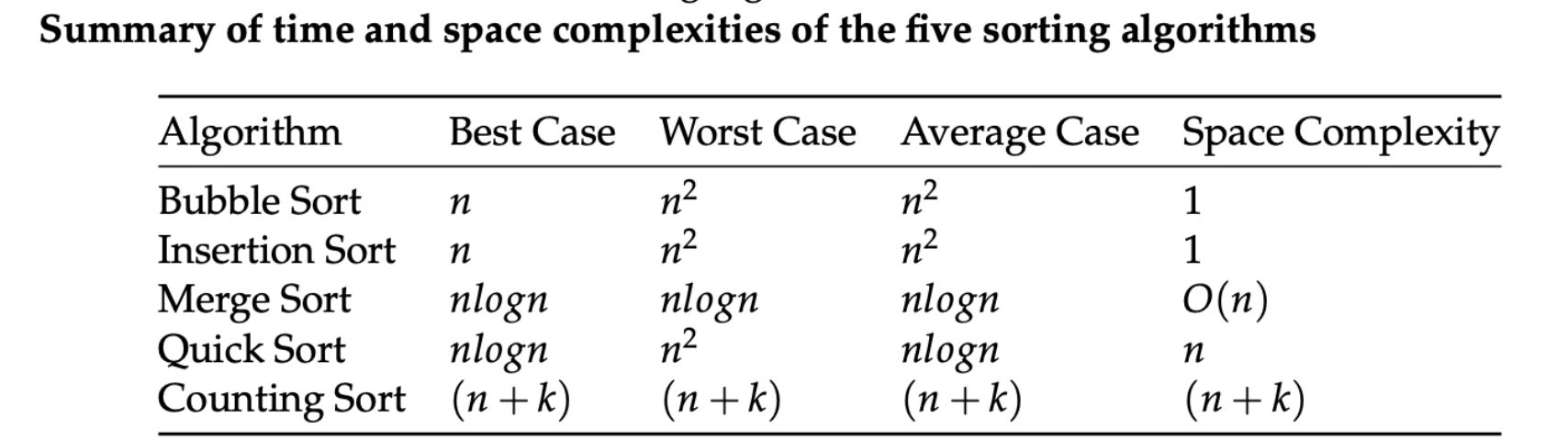
This section will give an overview of five sorting algorithms which are used in this benchmarking project and looks at their time and space complexities. Examples and diagrams are used to illustrate how each of the five algorithm works. Sample Python code to implement the algorithms is also included here.
In preparing this section, the same sources of information as in section 1 above was used. In addition various online resources were consulted for the Python code which are referenced below.
The five sorting algorithms introduced here are as follows:
- Bubble Sort as an example of a simple comparison-based sorting algorithm.
- Merge Sort as an example of an efficient comparison-based sorting algorithm.
- Counting Sort as an example of a non-comparison based sorting algorithm.
- Insertion Sort - another simple comparison-based sorting algorithm.
- Quick Sort - another efficient comparison-based sorting algorithm.
Bubble Sort: A Simple Comparison based sort
The following sources are referred to in this section.
- Computational Thinking with Algorithms lecture notes at GMIT.
- runestone interactive python
- wikipedia
- programiz,
- W3resources,
- geekforgeeks, runestone interactive python
Bubble Sort is a fairly simple comparison-based sorting algorithm and is so named for the way larger values in a list “bubble up” to the end as sorting takes place. The algorithm repeatedly goes through the list to be sorted, comparing and swapping adjacent elements that are out of order. With every new pass through the data, the next largest element bubbles up towards it's correct position. Although it is quite simple to understand and to implement, it is slow and impractical for most problems apart from situations where the data is already nearly sorted.
Bubble Sort works by repeatedly comparing neighbouring elements and swapping them if they are out of order. Multiple passes or iterations are made through the list and with each pass through the list, the next largest element ends up in it's proper place.
Bubble Sort begins by comparing each element in the list (except the very last one) with it's neighbour to the right, swapping the elements which are out of order. At the end of the first pass, the last and largest element is now in it's final place.
The second pass compares each element (except the last two) with the neighbour to the right, again swapping the elements which are out of order. At the end of the second pass through the data, the largest two elements are now in their final place.
The algorithm continues by comparing and swapping the remaining elements in the list in the same way, except those now already sorted at the end of the list. With each iteration the sorted side on the right gets bigger and the unsorted side on the left gets smaller, until there are no more unsorted elements on the left.
Example of Bubble Sort
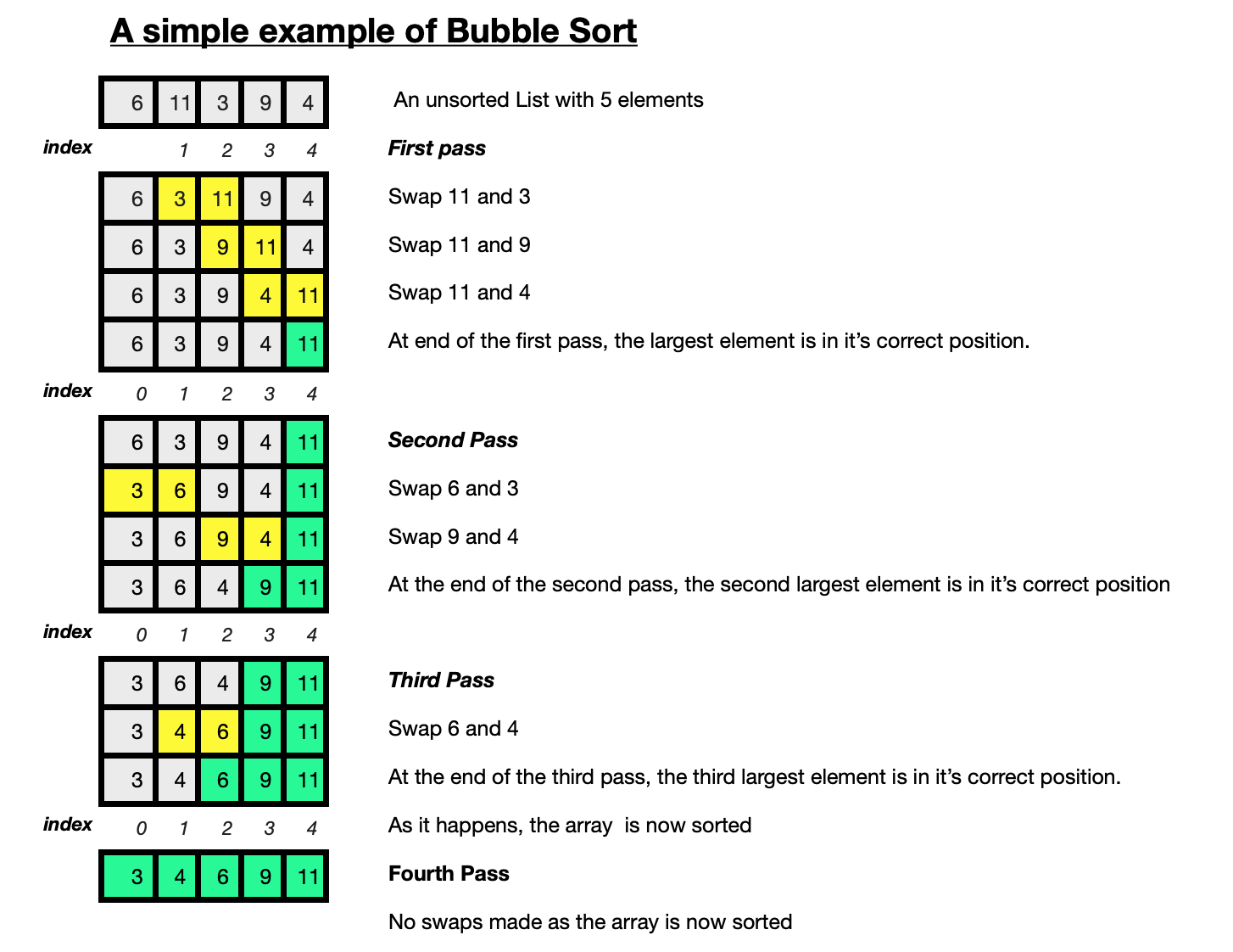
The above diagram illustrates how the Bubble Sorting algorithm works on a small array of 5 random numbers [6, 11, 3, 9, 4].
The example here shows how 4 ($n-1$) passes are made through the array of $n$ elements.
There are $n-1$ comparisons performed on the first pass, $n-2$ on the second pass, $n-3$ on the third pass and $n-4$ on the fourth and last pass.
The total number of comparisons is the sum of the first $n-1$ integers.
For the first pass, the algorithm iterates through the array from left to right, the first pair of elements that are out of order is (11,3) so the order of this pair is swapped and the array becomes [6, 3, 11, 9, 4]. Then the elements 11 and 9 are compared and swapped resulting in [6, 3, 9, 11 ,4], then 11 and 4 are swapped. At the start of the second pass, the array is now [6,3,9,11,4]. The first pair of elements to be swapped is (6,3)
- In the first pass, swaps are made between three pairs of elements:
(11, 3),(11, 9)then(11, 4). - At the end of the first pass the array is
[6, 3, 9, 4, 11]with the largest element11in its correct position. - In the second pass, swaps are made between two pairs
(6, 3)and(9, 4)resulting in[3, 6, 4, 9, 11]at the end of the second pass with the second largest element9now in it's correct place. - On the third pass through the list, there is only one pair to be swapped
(6,4). - At the end of the third pass, the array is sorted
[3, 4, 6, 9, 11]with each element in its correct sorted order. - Nevertheless the algorithm still does a fourth pass through the array, even though there are no more elements to be sorted.
- The algorithm is finished.
The python code to implement the Bubble Sort algorithm above is included here. This code is widely available online. The code used in this project was adapted from code at Runestone Academy: Problem Solving with Algorithms and Data Structures using Python. There is also an optimised version of the Bubble Sort algorithm known as the Short Bubble which stops early if the algorithm finds that the list has become sorted already before all the loops have executed.
Python code for Bubble Sort.
def bubbleSort(array):
    # loop n-1 times

    for passnum in range(len(array)-1,0,-1):
        # inner loop is shorted by 1 each time as another element is sorted
        for i in range(passnum):
            # comparing each element i with the element right beside it (i+1)
            if array[i] > array[i+1] :
                # swap out of order pairs so largest element is right of the smaller one
                array[i], array[i+1] = array[i+1], array[i]
A nested loop is used to compare each element and sort them into the correct place.
The outer loop for passnum in range(len(alist)-1,0,-1) starts from the second last element in the list and gets shorter each time, taking account of the fact that the elements at the end of the list are becoming sorted with each iteration of the outside loop. The inner loop goes through the elements, comparing the element on the left with the element on the right
Simultaneous assignment can be used instead of a temporary variable in Python when swapping the elements.
The outer loop runs $n-1$ times. At the end of each iteration, another element will be in it's final sorted position. The inner loop goes through each element in the array up to the element(s) already sorted, each time comparing each element $i$ with the element to the immediate right of it $i+1$.
Using the > comparison operator, the elements are compared. If the element on the left (at index i) is greater in value than the element on it's right (at index i+1) then the elements are swapped.
There are $n-1$ passes through a list of $n$ items. The total number of comparisons is the sum of the first $n-1$ integers which results in $n^2$ comparisons.
The best case occurs where the array is already sorted, as no exchanges are actually made however the comparisons still take place.
For the Bubble Sort algorithm, given an array that is almost or fully sorted it still requires $n-1$ passes through the input data. There is an optimised version of the Bubble Sort algorithm which can stop early.
The average case for the Bubble Sort algorithm is that exchanges are made half the time.
Analysing Bubble Sort.
The Bubble Sort algorithm here used two for loops where it first performs $n-1$ comparisons, then $n-2$ comparisons and so on down to the final comparison.
Illustrating the worst-case scenario for the algorithm which occurs when the array to be sorted is in sorted reverse order:
- given an array of
[5, 4, 3, 2, 1] - In the first pass, 4 swaps are made,
(5,4),(5,3),(5,2)and(5,1) - In the second pass 3 swaps are made
(4,3),(4,2)and(4,1) - In the third pass, the 2 swaps are made,
(3,2)and(3,1) - In the final pass, 1 swap is made,
(2,1). - In this case where all the elements were in reverse order, it tooks 10 swaps to sort the 5 element array.
For an array that is already sorted, for example [3,6,8,9,10] with 5 elements, there are still 4 loops through the array and comparisons made between all the pairs of elements, although no actual swaps are made.
In the worst case the outer loop has to execute $n-1$ times and in the average case the inner loop executes about $\frac{n}{2}$ times for each outer loop. Inside the inner loop, the comparison and swap operations take constant time $k$.
So it total it performs $(n-1) + (n-2) + (n-3) ... + 2+1$ which is $\frac{n^2}{2}+k \approx O(n^2)$.
(The constants $k$ which don't change with input size are removed which simplifies it to $n^2-n$, the $n$ is them removed as $n^2$ grows faster.)
The worst case scenario for Bubble sort occurs when the data to be sorted is in reverse order.
The Bubble Sort algorithm used here always runs in $O(n)$ times even if the array is sorted. There is a version of the algorithm which is optimised to stop if the inner loop didn't cause any swaps. If the optimised version of the Bubble Sort algorithm is applied on a nearly sorted array then the best case will be $O(n)$.
The average case is when the elements of the array are in random order.
The space complexity of Bubble Sort algorithm is $O(1)$. The only additional memory is needed for the variable used for the swapping.
Bubble sort is an in-place sorting algorithm and it is stable. It is not a very practical algorithm to use and is considered very inefficient as many exchanges are made before their final locations are known. It is possible to determine that the list is already sorted when no exchanges are made during the pass by modifiying the regular Bubble Sort algorithm.
Summary of time and space complexity of Bubble Sort:
- Best Case complexity: $O(n)$
- Average Case complexity: $O(n^2)$
- Worst Case complexity: $O(n^2)$
- Space complexity: $O(n)$
Merge Sort: An efficient comparison based sort
Merge Sort is an efficient, general-purpose, comparison-based sorting algorithm. This divide-and-conquer algorithm was proposed by John von Neumann in 1945 and uses recursion to continually split the list in half. A divide-and-conquer algorithm recursively breaks a problem down into two or more sub-problems of the same or related type until these become simple enough to be solved directly. Then the solutions to the sub-problems are combined to produce a solution to the original problem.
The list is divided into two evenly (as much as possible) sized halves which is repeated until the sublist contains a single element or less. Each sub-problem is then sorted recursively and the solutions to all the sub-lists are combined or merged into a single sorted new list. A list with one or less elements is considered sorted and is the base case for the recursion to stop. This algorithm will need extra memory to copy the elements when sorting. The extra space stores the two halves extracted using slicing.
Example of Merge Sort:
The diagram below demostrates how the MergeSort algorithm works on a small array of random integers [8, 6, 3, 4, 5, 2, 9].
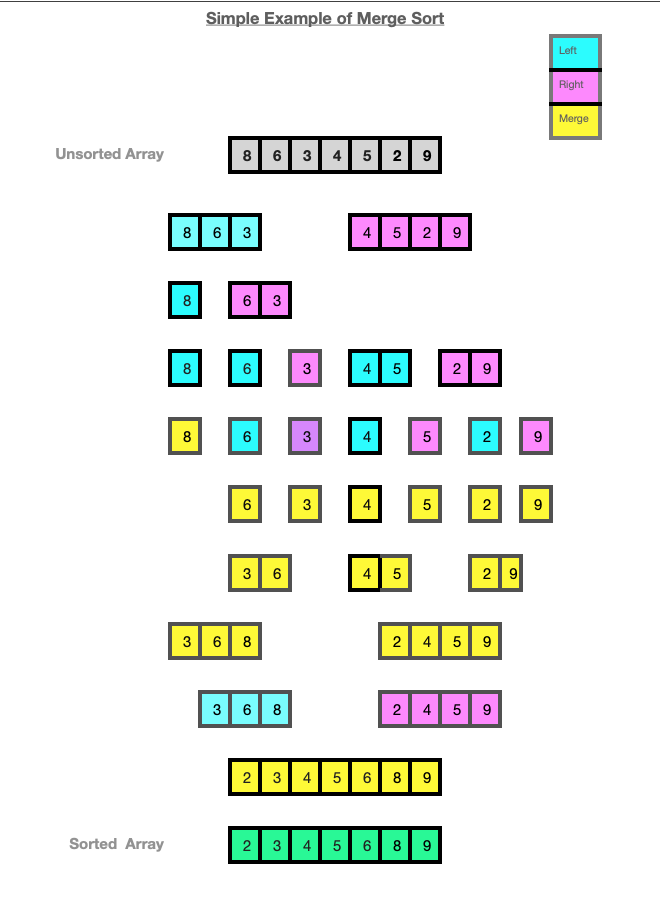
The array is split into a left array [8, 6, 3] and a right array [4, 5, 2, 9].
The left side of the array [8, 6, 3] is further split into [8] and [6, 3].
The [8] cannot be split any further so it is then ready to be merged. [6, 3] is split into [6] and [3] which are then ready to be merged.
[3] and [6] are then merged to become [3,6] and then they are merged with [8] resulting in a sub-array [3,6,8].
The right array [4, 5, 2, 9] is further split into [4,5] and [2,9] which are further split resulting in 4 sub-arrays [4],[5],[2] and [9]. The sub-arrays cannot be split any further and the merging begins. [4] and [5] are merged into [4,5].
[2] and [9] are merged into [2,9]. The two sorted sub-arrays [4,5] and [2,9] are then merged to become [2, 4, 5, 9].
The sorted sub-array [3,6,8] is then merged with the sorted right array [2, 4, 5, 9].
The result is a single sorted array of [2, 3, 4, 5, 6, 8, 9].
The colours blue and pink are used to show the arrays being split or sub-divided into left and right arrays. The colour yellow is used to show the merge operation which takes place after the splitting of each sub-list is complete.
Python code for Merge Sort
The following is the python code for the Merge Sort algorithm. This code is widely available online. The code used in this project is from Runestone Academy.
def merge_sort(array):

    if len(array)>1:
        # find the middle of the list to get the split point
        mid = len(array)//2
        # left contains the elements from the first half of the list
        left = array[:mid]
        # right contains the elements from the second half of the list
        right = array[mid:]
        # recursively call the function on the first half
        merge_sort(left)
        # recursively call the function on the second half
        merge_sort(right)


        i ,j, k = 0,0,0 # index of the left, right and merged arrays

        while i < len(left) and j < len(right):
       # compare next element, place smaller element next into sorted array

            if left[i] <= right[j]:
                array[k]=left[i]
                # next comparison
                i += 1
            else:
                array[k]=right[j]
                # next comparison
                j += 1
            # after assigning another element to the merged array, increment the index by 1
            k=k+1
        # if no elements left in right array, move any elements in left to merged array
        while i < len(left):
            array[k]=left[i]
            i += 1
            k += 1
        # no elements left in left array, move any elements in right array to merge
        while j < len(right):
            array[k]=right[j]
            j += 1
            k += 1
    return array
The recursive divide-and-conquer approach results in a worst-case running time of $O(n\log{}n)$ for the Merge Sort algorithm. The algorithm consists of two distinct processes, the splitting and the merging.
- A list can be split in half $\log n$ times where $n$ is the number of elements in the list.
- Each item in the list will eventually be processed and placed in the sorted list. This means a list of size $n$ will require $n$ operations. Therefore there are $\log n$ splits, each of which costs $n$ for a total of $n \log n$ operations
- Merge Sort needs extra space to hold the left and right halves which can be a critical factor for large datasets.
Merge-Sort has a similar best, worst and average cases of linearithmic $n\log{}n)$ time complexity in each case which makes it a good choice if predictable run-time is important. There are versions of Merge Sort which are particularly good for sorting data with slow access times such as data that cannot be held in RAM or are stored in linked lists.[3] Merge Sort is a stable sorting algorithm.
Summary of time and space complexity of Merge Sort
- Best Case complexity: $O(n\log{}n)$
- Average Case complexity: $O(n\log{}n)$
- Worst Case complexity: $O(n\log{}n)$
- Space complexity: $O(n)$
Counting Sort: A non comparison sort
See W3resources,Wikipedia, Programiz.com, GeeksForGeeks.com.
The Counting sort algorithm which was proposed by Harold H. Seward in 1954, is an algorithm for sorting a collection of objects according to keys that are small integers. It is an integer sorting algorithm that counts the number of objects that have each distinct key value, and using arithmetic on those counts to determine the positions of each key value in the output sequence.
While comparison sorts such as Bubble Sort and Merge Sort make no assumptions about the data, comparing all elements against each other, non-comparison sorts such as Counting Sort do make assumptions about the data, such as the range of values the data falls into and the distribution of the data. In this way the need to compare all elements against each other is avoided. Counting Sort allows for a collection of items to be sorted in close to linear time which is made possible by making assumptions about the type of data to be sorted.
The Counting Sort algorithm uses keys between a specific range and counts the number of objects having distinct key values. To implement it you first need to determine the maximum value in the range of values to be sorted which is then used to define the keys. The keys are all the possible values that the data to be sorted can take. An auxillary array is created to store the count of the number of times each key value occurs in the input data.
Example of Counting Sort Algorithm:
The Counting Sort algorithm sorts the elements of a list by counting the number of occurences for each unique element in the list. This count is stored in another counter array. The sorting is performed by mapping the count as an index of the counter array.
Go through the array of input data and record how many times each distinct key value occurs. The sorted data in then built based on the frequencues of the key values stored in this count array.
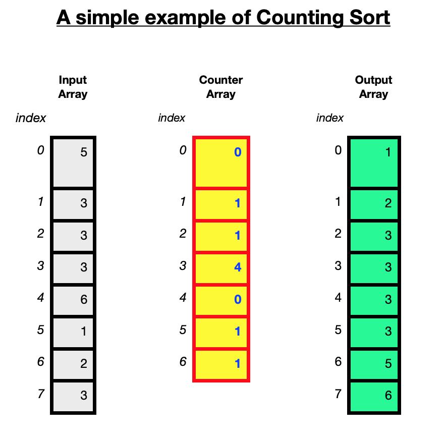
The diagram above illustates how the counting sort algorithm works using an unsorted array of 8 integers [5, 3, 3, 3, 6, 1, 2, 3].
The maximum value in the array is 6.
The algorithm takes an unsorted array of elements. The maximum value is used to create a counter array. The purpose of the counter array is to hold the number of times each element occurs in the input. In this case a counter array is created with 7 elements to record how often the 7 integers from 0 to 6 occur in the array. This can be initialised with zeros.
The algorithm goes through the input data, using the value of the element to go to the position with this index in the counter array. For example if it comes across the value 3 in the array to be sorted, go to index 3 of the counter array and increment the value in index 3 by 1. If the value 3 is encountered again, increment the value of the counter at index 3 by 1. This records the number of times the number 3 occurs in the input data. Once this is done for all elements in the input array, the counter will hold the number of times each unique element has occured. [0, 1, 1, 4, 0, 1, 1]
This counter array is then used to place the elements into a sorted array.
The first element in the counter array represents how many times the number 0 occured in the input array, the second element represents how many times the number 1 occured in the array, the 3rd element in the counter represents how many times the number 2 occured in the array and so on.
The counter array [0, 1, 1, 4, 0, 1, 1] shows that there are zero 0's, one 1, one 2, four 3's, zero 4's, one 5 and one 6.
The numbers are then placed into the sorted array in order as follows:
Wherever the counter element is greater than 0, place the number it is holding count for into the sorted array that many times.
So the output array will have [1,2,3,3,3,5,6]
If an array contained larger values, then this would result in a larger counter array being created. For example if the array contained values up to say 9,999 then the counter would be of size 10,000 which would result in a much longer time spent iterating over a larger counter array.
Python code for Counting Sort:
The Python code for the Counting Sorting algorithm is widely available online at w3resources.com, geeksforgeeks, programiz.
I have slightly adapted the variable names for my own understanding and commented the code.
def CountingSort(array):
    n= len(array)
    # a counter array initialised with zeros,
    counter= [0 for i in range(max(array)+1)]
    sorted = []   #to store the sorted values
    # loop over elements, use the element of input as the index for the counter
    for i in array:
        # each time an element appears in the array, increment the counter by 1
        counter[i] += 1
    # Use count of each element occurs to place elements in the sorted array

    for i in range(0,len(counter)):
        # while the counter shows that there is a matching element
        while counter[i] > 0:
            # append the element to the sorted array
            sorted.append(i)
           # decrease the counter by 1 each time
            counter[i] -= 1
    return sorted
The Time and Space Complexity of the Counting Sort Algorithm
The Counting Sort algorithm allows for the sorting of a collection of items in close to linear time. $O(n)$ time is possible because assumptions can be made about the data and therefore there is no need to compare elements against each other as there is with the comparison based algorithms mentioned earlier.
The input to the Counting Sort algorithm is generally a collection of $n$ items with each item having a non-negative integer key with a maximum value of $k$, or just a sequence of integers.
The range of values could be determined both inside the algorithm or outside of the algorithm and provided as a parameter to the function.
There are no comparisons at all made between any elements.
The best, worst and average complexities will always be the same because it doesn't matter what order the elements are in the array to be sorted, the algorithm will still have to iterate $n+k$ times where $n$ is the size of the array to be sorted and $k$ is the largest value in the array which determines the size of the counter array.
The space complexity depends on the maximum value in the data to be sorted. A larger range of elements requires a larger counter array.
The counting sort algorithm is a stable sorting algorithm if it is implemented in the correct way. As the algorithm iterates over the elements again placing them into their sorted position in the output array, the relative order of the items with equal keys is maintained.
Counting Sort is considered suitable for use only with smaller integers which have multiple counts. This is demonstrated in the example above.
wikipedia summarises it best: counting sort's running time is linear in the number of items and the difference between the maximum and minimum key values, so it is only suitable for direct use in situations where the variation in keys is not significantly greater than the number of items. However, it is often used as a subroutine in another sorting algorithm, radix sort, that can handle larger keys more efficiently.
Summary of time and space complexity of Counting Sort
- Best Case complexity:$n + k$
- Average Case complexity:$n + k$
- Worst Case complexity: $n + k$
- Space complexity: $n + k$
Insertion Sort.
Insertion Sort is a simple comparison-based algorithm.
See interactive python, w3resources, programiz, realpython, Wikipedia
According to Wikipedia, Insertion sort is a simple sorting algorithm that builds the final sorted array (or list) one item at a time. It is much less efficient on large lists than more advanced algorithms such as quicksort, heapsort, or merge sort.
The Insertion Sort algorithm is relatively easy to implement and understand as it can be compared to sorting a deck of cards. The first element is assumed to be sorted. The sorted list is built one element at a time by comparing each item with the rest of the items in the list, then inserting the element into its correct position. After each iteration, an unsorted element has been placed in it's right place.
Insertion Sort is an iterative algorithm. The basic steps for the Insertion Sort algorithm are as follows.
Starting from the left of the input array, set the key as the element at index 1. As a list with a single element is considered sorted, the very first element at index 0 is skipped.
Comparing any elements to the left of this key with the key, move any elements which are greater in value than the key right by one position and insert the key. Next move to the element at index 2 and make this the key and in the same way moving any elements on the left of the key that are greater than the key to the right by one position.
Repeat this with all the elements up to the last element. There is one pass through the list for every element from index 1 to index $n-1$
At each pass the current key element is being compared with a (growing) sorted sublist to the left of it. Any elements with a value greater than the key is moved to the right each time. After this process the array should be sorted..
After k passes through the data, the first k elements of the input data are in sorted order.
Example of Insertion Sort
The diagram below illustrates how the Insertion Sort algorithm works on a small array of random integers a=[6,11,3,9,4].
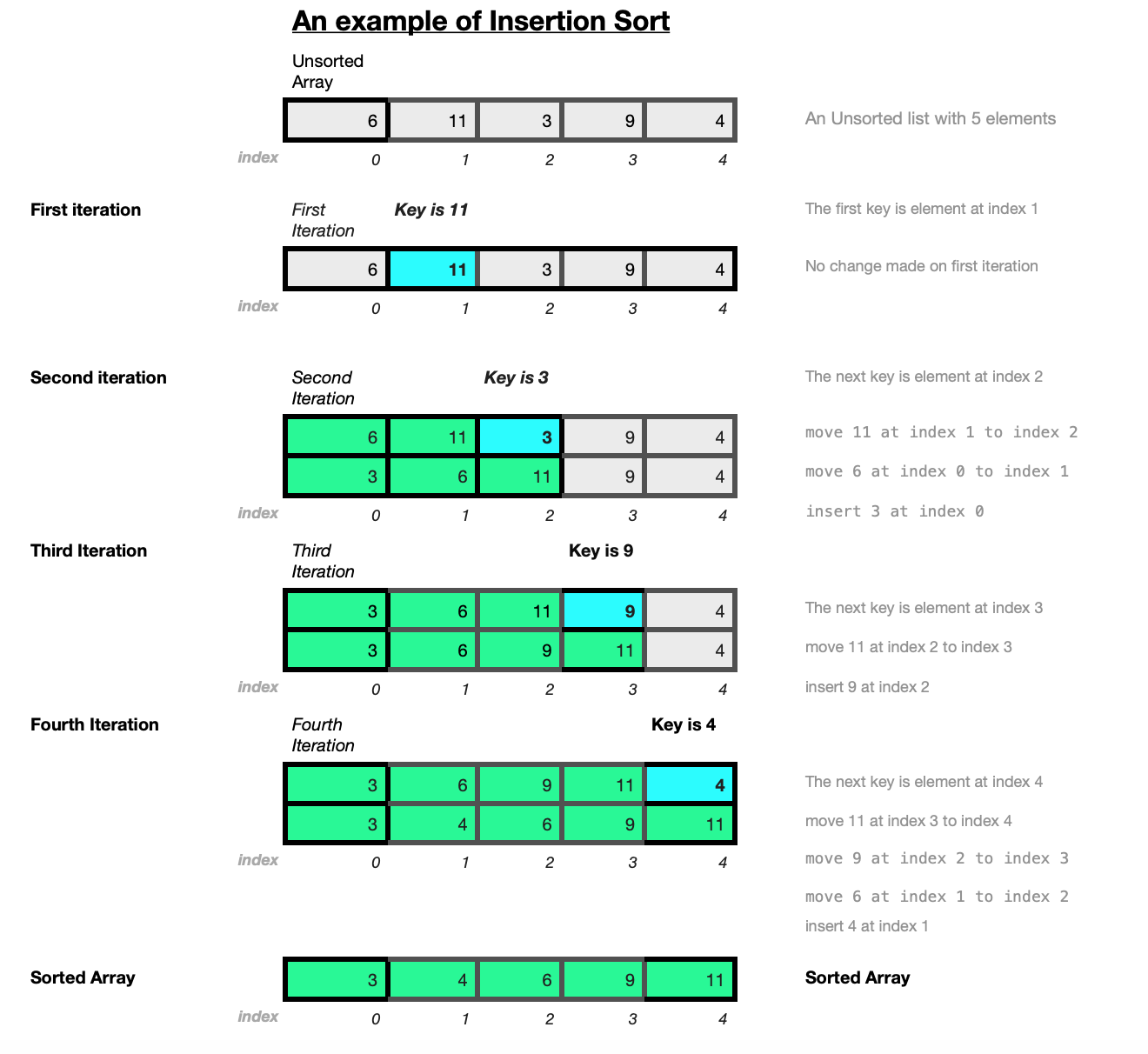
In the example,the algorithm takes the unsorted array a=[6,11,3,9,4].
The first key is the element at index a[1] which is 11. Looking to the element to it's left at a[0], 11 is greater than 6, there is no exchange required.
The next key is the element at a[2] which is 3. Comparing 3 to the element on it's left 11 at a[1], as 11 is greater than 3, 11 is moved from a[1] to a[2]. The element 6 at a[0] is moved to a[1].
At the beginning of the second iteration we have [6, 11, 3, 9, 4].
The key is the element at a[2] which is 3 which is less in value than the elements on it's left. Therefore 11 is moved from a[1] to a[2] and 6 is moved from a[0] to a[1]. The key element 3 is then inserted at a[0].
At the beginning of the third iteration, the array is now [3, 6, 11, 9, 4]. The key is the element at position 3 which is 9. Comparing to the elements on the left of it, 11 is moved from a[2] to a[3] and 9 is inserted at position 2 resulting in
[3, 6, 9, 11, 4] at the beginning of the fourth iteration. The fourth key is the element 4 at a[4]. Comparing to the elements to it's left, 11 is moved from a[3] to a[4] and 9 is moved from a[2] to a[3], 6 is moved from a[1] to a[2]. Then the key 4 is inserted into the array at a[1] resulting in array [3, 4, 6, 9, 11] which is now sorted.
Python Code for Insertion Sort.
The Python code for the Insertion Sort algorithm is widely available online at Runestone Academy, W3resources.com,Programiz.com among others. I have slightly adapted the variable names here for my own understanding and commented the code. (This code can be slightly amended to sort in descending order.)
def insertionSort(array):
    # start at index 1
    for i in range(1,len(array)):
    # iterate through the array, each time the next element is the key
        key = array[i]
    # initialise j element left of the current key
        j = i -1
    # while key is < than elements to on left, move all elements > key right by one
        while j >= 0 and array[j] > key:
            array[j+1] = array[j]
         # j to point to the next element
            j -= 1

    # then move key to its correct new position after the element just smaller than it.
        array[j+1]=key
Analysing Insertion Sort
There are $n-1$ iterations required to sort $n$ items with an iteration for each element from the second element at index 1 up to the last element.
In the best case only one actual comparison is required on each iteration. The best case would occur on a list that is already sorted. The inner loop does not need to iterate at all on a list that is already sorted.
Insertion sort is the only comparison-based sorting algorithm that does this. The inner loop only iterates until it finds the insertion point.
Here is an example of best case using a small sorted array [6, 7, 8, 9, 10].
The first key is 7 at index 1, the element 6 before it at index 0 is smaller than 7 so no move is required. The next key 8 at index 2 is greater than the element before it at index 1. In the same way there is no move required for key 9 at index 3 and key 10 at index 4.
On input data sets that are almost sorted, the Insertion Sort algorithm runs in $n + d$ time where $d$ is the number of inversions. An inversion is a pair of index positions where the elements are out of order. A sorted list would have no inversions and therefore run in linear time in the best case.
On average a list of size $n$ has $\frac{(n-1)n}{4}$ invertions and $n-1 + \frac{(n-1)n}{4} \approx n^2$ comparisons.
The Insertion Sort algorithm is not very efficient on large random datasets. In the worst case where all items are in reverse sorted order, a list of size n has $\frac{(n-1)n}{2}$ invertions. The maximum number of comparisons then would be $n-1 + \frac{(n-1)n}{2} \approx n^2$
This is the sum of the first $n-1$ items which is $n^2$.
Worst-case example:
Illustrating the worst case scenario on a small array of elements sorted in reverse order [8,6,4,3,2].
The first key 6 at index 1 is smaller than the previous element at index 0 so 8 is moved from index 0 to position 1, the key 6 is inserted at position 0 resulting in [6, 8, 4, 3, 2] for the second iteration. The next key 4 at index 2 is smaller than 8 in index 1 so 8 is moved to index 2, 6 is moved from index 0 to index 1. The key 4 is then inserted into index 0.
At the start of the third iteration we have [4, 6, 8, 3, 2], the key is now the value 3 at index 4 which is less than the element before it, 8 at index 2. Therefore 8 is moved from index 2 to index 3, 6 is moved from index 2 to index 1, 4 is moved from index 0 to index 1 and the key 3 is inserted into index 0.
At the fourth and final iteration, the array is now [3, 4, 6, 8, 2], the key is 2 at index 4 which is less than all the elements before it. Therefore 8 is moved from index 3 to index 4, 6 is moved from index 2 to index 3, 4 is moved from index 1 to index 2, 3 is moved from index 0 to index 1 and the key is inserted at index 0 resulting in a sorted array in ascending order.
In the best case, on an list that is already sorted the inner loop does not need to iterate at all.
The space complexity is $O(1)$ because of the additional variable key being used.
The Insertion Sort differs from other simple sorting algorithms such as Bubble Sort and Selection Sort in that while values are shifted up one position in the list, there is no exchange as such. Runestone Academy notes that in general, a shift operation requires approximately a third of the processing work of an exchange since only one assignment is performed.
Therefore in benchmark studies such as this, Insertion Sort should show very good performance compared to other simple sorting algorithms such as Bubble Sort.
Insertion Sort is a stable in-place sorting algorithm. It works well on small lists and lists that are close to being sorted but is not very efficient on large random lists. It's efficiency increased when duplicate items are present.[2]
Summary of time and space complexity of Insertion Sort
- Best Case complexity: $O(n)$
- Average Case complexity:$(n^2)$
- Worst Case complexity: $(n^2)$
- Space complexity: $1$
Quick Sort
See Runestone Academy,W3resource.com, Wikipedia, geeksforgeeks, programiz.com
The Quick Sort algorithm is somewhat similar to Merge Sort as it a comparison-based algorithm that uses a recursive divide-and-conquer technique. It does not however need the extra memory that Merge Sort requires. A pivot element is used to divide the list for the recursive calls to the algorithm.
The Quicksort algorithm was developed by Tony Hoare in 1959. According to Wikipedia the QuickSort algorithm is also known as the partition-exchange sort and when implemented well, it can be about two or three times faster than its main competitors, merge sort and heapsort.
A pivot element is used to divide the list for the recursive calls to the algorithm. This is an element chosen from the array to be sorted. Any element from the array can be chosen as the pivot element but usually one of the following four options is used.
- pick the first element as the pivot
- pick the last element as the pivot
- pick a random element as the pivot
- pick the median element as the pivot. The pivot chosen can determine the performance.
The key part of the quick sort algorithm is the partitioning which aims to take an array, use an element from the array as the pivot, place the pivot element in its correct position in the sorted array, place all elements that are smaller than the pivot before the pivot and all the elements that are larger than the pivot after the pivot element.
A pivot element is chosen, elements smaller than the pivot are moved to the left while elements greater than the pivot are moved to the right. The array elements are reordered so that any array elements less than the pivot are placed before the partition while array elements with values greater than the pivot element come after. After the partioning, the pivot will be in it's final position
Example of Quick Sort
The main steps in the quicksort algorithm are shown in the example below.
- Select a
pivotfrom the array. Partitioning: Any elements smaller than the
pivotare put to the left of the pivot, and any elements greater than the pivot are moved to the right.
Reorder the array elements with values less than the pivot to be before the partition, the array elements with values greater than the pivot element come after the partition. After the partioning, the pivot will be in it's final positionRecursion is used to apply the above two steps recursively to each of the two sub-arrays.
Example illustrating how the Quick Sort Algorithm works.
The diagram below illustrates how the Quick Sort algorithm works on a small array of random integers [54,25,92,16,76,30,43,55,20]. In this example the first element is used as the pivot value for partitioning.
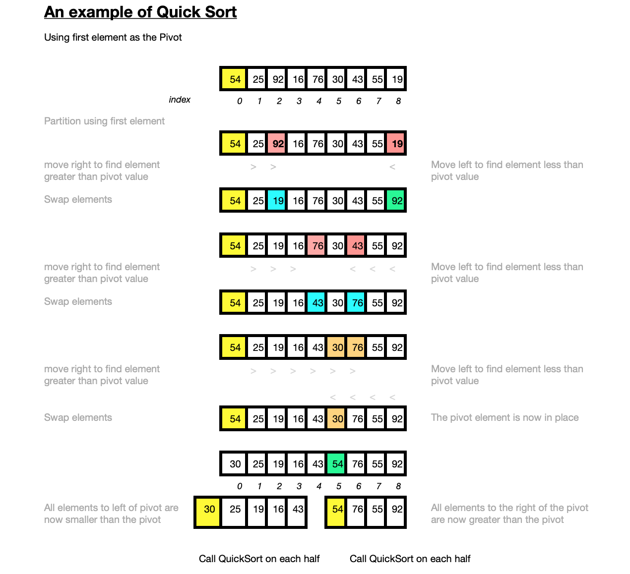
The first pivot element is 54 at index 0. The algorithm places a pointer at the next element 25 and passes over the elements in the array from left to right until it finds the first element which is greater than the pivot value, in this case 92. Another pointer is placed at the very last element in the array. Moving left from this position until the first element is found that is less than the pivot value. This is the very last element itself 92. The two out of place elements are swapped resulting in [54,25,20,16,76,30,43,55,92]. Again moving right until the first element greater than the pivot value is found 76 while moving left from the last element until the first element less than the pivot is found at 43. This results in the values 76 and 43 being swapped. Starting again from the pivot [54,25,20,16,43,30,76,55,92] and moving right to find the first element greater than the pivot which is 76. At the same time moving left from the end of the array to find the first element less than the pivot is 30. However as the first value smaller than the pivot (from the end of the array) is positioned before the first value greater than the pivot from the beginning, the algorithm stops. The pivot value 54 is swapped with the value 30 resulting in [30,25,20,16,43,54,76,55,92]. The pivot value is now in it's correct and final position in the sorted array.
All elements to the left of the pivot value 30,25,20,16,43 are now less than the pivot value, all elements to the right of the pivot [76,55,92] are greater than the pivot. A split point has therefore been found. The QuickSort algorithm is then recursively called on the two halves [30,25,20,16,43] and [76,55,92] using the first element in each subarray as the pivot.
Taking the first half [30,25,20,16,43], the first pivot is 30, then once it is placed in it's final position the pivot of the next sub-array [16,25,20] is 16, the next pivot is 25.
The first pivot on the right sub-array [76,55,92] is 76, once this is in place the sub-array is sorted. The sorted sub-arrays are then joined together resulting in sorted array
[16, 20, 25, 30, 43, 54, 55, 76, 92]
Python code for QuickSort algorithm:
The Python code for the Quick Sort sorting algorithm is widely available online. The code here is from Interactive python
Quick Sort is a recursive algorithm. The base case for the recursion is a subarray of length 0 or 1 as any such array will be considered sorted. The first element in this implementation is used as the pivot for partitioning.
def quickSort(array):
    # call a recursive function that takes in the array,
    quickSortHelper(array,0,len(array)-1)
    return array

# if length of list passed in is > 1, partition the array and recursively sort
def quickSortHelper(array,first,last):
    if first<last:
        splitpoint = partition(array,first,last)  # find the split point
        # recursively call the function on the two halves of the array
        quickSortHelper(array,first,splitpoint-1)
        quickSortHelper(array,splitpoint+1,last)

# a function to partition the array using the pivot element,
def partition(array,first,last):
    # the pivot is the first element in the array
    pivotvalue = array[first]
    # the first pointer is the first element in the remaining unsorted part
    leftmark = first+1
    # the right pointer is the last element remaining
    rightmark = last

    done = False
    while not done:
        # move the first pointer right until the first element > pivot is found
        while leftmark <= rightmark and array[leftmark] <= pivotvalue:
            leftmark = leftmark + 1
        # move the second pointer left until the first element < pivot
        while array[rightmark] >= pivotvalue and rightmark >= leftmark:
            rightmark = rightmark -1
        # stop when the second pointer is less than the first pointer (when cross over)
        if rightmark < leftmark:
            done = True
        else:
           # using simulataneous assignment to swap the values that are out of place
            array[leftmark],array[rightmark]  = array[rightmark], array[leftmark]
    # swap with the pivot value
    array[first],array[rightmark] = array[rightmark],array[first]

    return rightmark
The worst-case scenario for Quick Sort depends on the chosen pivot point. If the partition process always picks the smallest or greatest element as the pivot.
The worst case occurs when the array to be sorted is already sorted in the same order or in reverse order or if all elements are the same. geekforgeeks describes how if a random element or a median element is instead chosen for the pivot the worst cases are unlikely to occur unless the maximum or minimum element happens to always be selected as the pivot. The best case occurs when the partition process always picks the median value as the pivot.
In practice it is one of the fastest known sorting algorithms, on average. While memory usage is $O(n)$, there are variants of the Quick Sort algorithm that are $O(n\log n)$
Standard version is not stable, although stable versions do exist.
According to Wikipedia Inefficient implementations it is not a stable sort, meaning that the relative order of equal sort items is not preserved. Quicksort can operate in-place on an array, requiring small additional amounts of memory to perform the sorting.
Summary of time and space complexity of Quick Sort
- Best Case complexity: $O(n\log n)$
- Average Case complexity:$O(n\log n)$
- Worst Case complexity: $O(n^2)$
- Space complexity: $O(n)$.
Implementation and Benchmarking
In this section I will describe the process using for implementing my Python application for this project before presenting the results.
The purpose of the application is to benchmark the five different sorting algorithms introduced above in section 2.
Sorting Algorithms used:
- Bubble Sort - A simple comparison-based sorting algorithm
- Merge Sort - An efficient comparison based sorting algorithm
- Counting Sort - A non-comparison based sorting algorithm.
- Insertion Sort - another simple comparison based sorting algorithm
- Quick Sort - Another efficient comparison based sort.
The results of the benchmarking will be presented in a table and a graph. The performance of each algorithm is then reviewed in relation to the expected time complexity for each one as outlined above in section 2 and with respect to each other.
The main Python application used for the benchmarking of five sorting algorithms is called benchmarking.py.
The purpose of the application is to take arrays of randomly generated integers of varying input sizes and to test the effect of the input size on the running time of each sorting algorithm. The running time for each algorithm is measured 10 times and the averages of the ten runs for each sorting algorithm and for each input size is then output to the console when the program has finished executing. The application also generates a plot of the resulting averages. The elapsed times for each individual run for each type of algorithm of each input array size are exported to csv file for reference. The average times are also exported to another csv file.
The Python code for the actual sorting algorithms are written in separate Python .py script files and imported as modules to the benchmarking program. As outlined in section 2 above, the codes used for these sorting algorithms are widely available online.
Python's random module was used to create random array sizes that varied from 100 integers to 10,000 integers.
The time function from the time module function records time in seconds from the epoch.
pandas
The main benchmarking function benchmarking takes in three arguments.
- The first argument is a dictionary containing the names of the sorting algorithms and the name of the module it is in.
- The second argument is array containing the different input sizes.
- The last argument is the number of runs to run each sorting algorithm.
The program consists of an outer for loop which iteratates through each of the different sorting algorithms provided to it, a nested for loop which iterates through each of the sizes in the size arrays and another nested for loop which iterates the number of times provided to the runs parameter. Within the inner for loop, a new random array is created each time using the size as the number of random elements. Each sorting function is called 10 times for each different size array. A new random array is created each time.
The time function from the time module is used to time the actual sorting function applied to the random array generated. The [time.time]
(https://docs.python.org/3/library/time.html#time.time) function returns the time in seconds since the epoch as a floating point number.
The time is taken immediately before the sorting function sorts the data and immediately after the sorting function sorts the data. The elapsed time is calculated as the difference between the two times. The creation of the random array itself is not timed.
At each run, the elapsed time, the run number (1 to 10), the name of the sorting function and the size of the input array sorted each time is recorded in lists. The results of each trial for each type of sorting algorithm for each input size to be sorted is then output to a pandas dataframe. This contains the results of each individual trial in seconds. Another function is then called by the main program which takes the dataframe containing the raw elapsed times and calculates the averages to 3 decimal places of the 10 different runs for each sort algorithm for each input size. The pandas groupby function is used here to get the averages grouped by the sorting function name and the input array size. The results are multiplied by 1000 to get the averages in milliseconds. The results of the groupby operation is then unstacked to get the results in the desired format for this benchmarking project.
The main function also calls another function to plot the averages using the matplotlib.pyplot module and the seaborn library resulting in a graph showing the average times in milliseconds on the vertical axis and the size of the input array on the horizontal axis.
When testing the program, print statements were used to ensure that the resulting dataframe of elapsed times did indeed contain the correct elapsed time for each trial for each algorithm at each input size. The dictionary of sorting algorithms could be changed to test the performance of a single sorting algorithm or a combination of algorithms. The
Python Benchmarking application code
Benchmarking.py saved in script folder with the sorting algorithms saved in the same folder.
import random
import time
import pandas as pd
import numpy as np
import bubble
import merge
import counting
import insertion
import quick

import matplotlib.pyplot as plt

# runs the benchmarking,
def benchmarking(algorithms, Sizes, runs):
    # create some variables to append the output to
    elapsed_times = [] # this should end up with 10 elapsed times for each innermost loop
    input_size =[] # to record the array size used for each run
    trials =[] # to record the current trial number for each algorithm
    type =[] #  to record the name of the sorting algorithm used


    # for each of the 5 sorting algorithms
    for sort_algo in algorithms:
        print(f"running {sort_algo}")
        # for each array size in the size array
        for size in Sizes:
            # run this 10 (runs) times for each size for each sort type
            for run in range(runs):
                # generate random arrays
                x = [random.randint(0,100) for i in range(size)]

                #print(f" function {sort_algo} on array of length {len(x)}")
                # select the sorting algorithm to use
                algorithm = algorithms[sort_algo]
                # time.time return the time in seconds since the epoch as a floating point number
                start_time = time.time()
                # run the actual algorithm on the current run on the current array size
                algorithm(x)
                end_time = time.time()
                time_elapsed = (end_time - start_time)* 1000 # to get milliseconds

                # record the results of current test to the results array
                elapsed_times.append(time_elapsed)
                # record the current run number (from 1 to 10)
                trials.append(run+1)
                # record the current size to the input size array
                input_size.append(size)
                # record the name of the current sorting algorithm
                type.append(sort_algo)

    # outputs a dataframe with the raw times for each trial
    df = pd.DataFrame({"Sort":type, "Size":input_size, "Times":elapsed_times, "trialNo":trials})
    return df

# Define a function to take the output of the benchmarking function and calculate the averages
def mean_sorts(df):
    # use the Size column of the dataframe as the index
    df.set_index('Size', inplace=True)
    # calculate the averages for each sorting algorithm at each level of input size
    means = (df.iloc[:, 0:2].groupby(['Sort','Size']).mean()).round(3)
    # unstack the dataframe to get the desired format for the output to the console
    return means.unstack()

# define a function to plot the averages on a graph
def plot_averages(df2):
    # import plotting libraries
    import seaborn as sns
    import matplotlib.pyplot as plt
    # set the plot paramters
    plt.rcParams["figure.figsize"]=(16,8)
    sns.set(style= "darkgrid")
    # transpose the dataframe for plotting
    df2.T.plot(lw=2, colormap='jet', marker='.', markersize=10,
         title='Benchmarking Sorting Algorithms - Average Times')
    plt.ylabel("Running time (milliseconds)")
    plt.xlabel("Input Size")
    #plt.ylim(0,80)
    #plt.show()
    # save image
    plt.savefig('plot100.png', bbox_inches='tight')

# define a function to export the results to csv
def export_results(times, means):
    # change this to store in a different file each time so I can compare results
    times.to_csv('xxxTime_trials' + '100'+'.csv')
    means.to_csv('xxxAverages' + '100' + '.csv')

# call the main program
if __name__ == "__main__":
    # the list of algorithms to be used
    algorithms = {"BubbleSort": bubble.bubbleSort,"insertionSort":insertion.insertionSort,"mergeSort":merge.merge_sort, "quickSort":quick.quickSort, "CountingSort": counting.CountingSort}
    # provide the sizes for the arrays to be sorted
    sizeN = [250,500,1000]
    sizeN = [100,250,500,750,1000,1250,2500]

    # call the benchmarking function
    results = benchmarking(algorithms, sizeN, 5)

    print("The running time for each of the 5 sorting algorithms have been measured 10 times and the averages of the 10 runs for each algorithm and each input size are as follows \n ")
    # create a dataframe to store the averages resulting from the benchmarking
    df2=  mean_sorts(results)
    # drop 'Sort'
    df2.rename_axis(None, inplace=True)
    # drop one of the multi-index levels
    df2.columns = df2.columns.droplevel()
    # print the results to the console
    print(df2)
    # call the plotting function
    plot_averages(df2)
    # export the results to csv
    export_results(results, df2)
Results of the Benchmarking on the five sorting algorithms.
The results of the benchmarking using the code above is presented here.
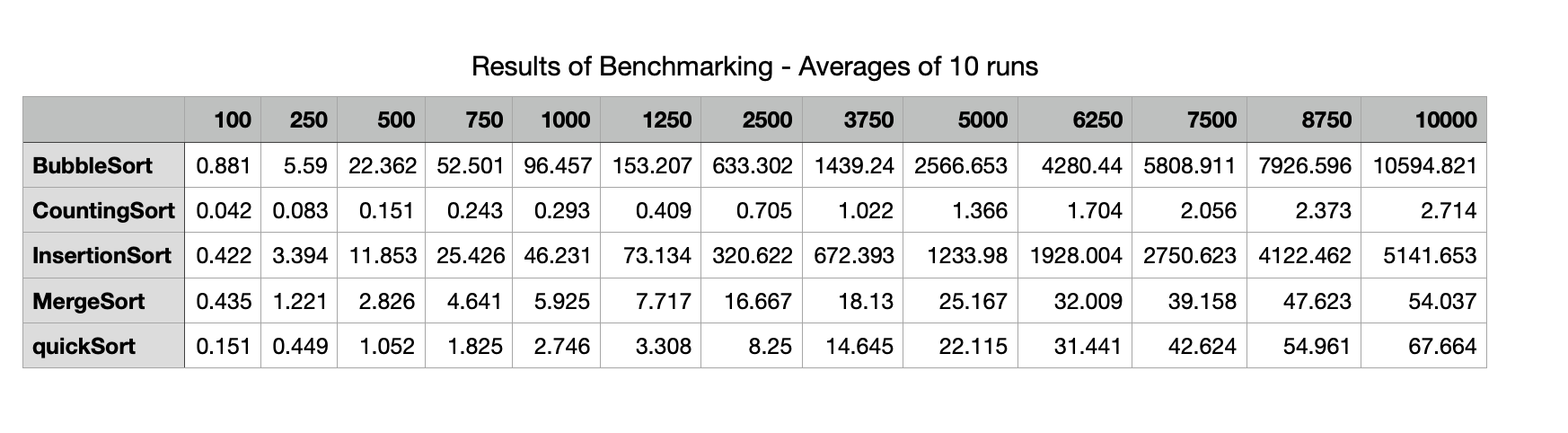
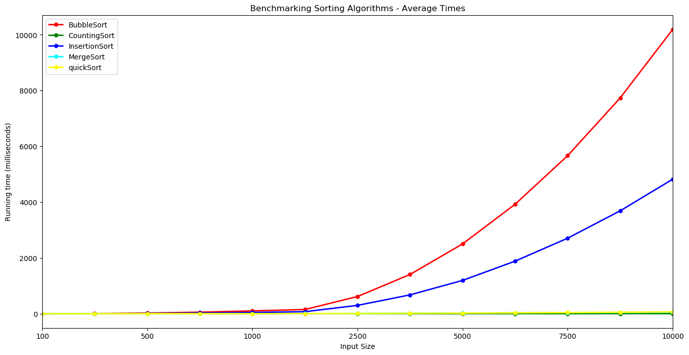
The results of the benchmarking using the code above is presented here. The table shows the average times in milliseconds across the 10 runs for each sorting algorithm using the different sized inputs from 100 elements up to 10,000 elements. The table shows that Bubble Sort takes over 10 seconds to sort a random array containing 10,000 random integers while Counting Sort performs the same task in less than 3 milliseconds. Insertion Sort here takes about half the time as Bubble Sort. Merge Sort and Quick Sort and Merge Sort have times of the same order. The plots illustrate the performance of the five sorting algorithms and how they differ from each other. Bubble Sort increases at a faster rate, followed by Insertion Sort. These algorithms display an $n^2$ growth rate. It is hard to distinguish Counting Sort, Merge Sort and Quick Sort here given the scale of the y-axis which is dominated by the very slow times for Bubble Sort.
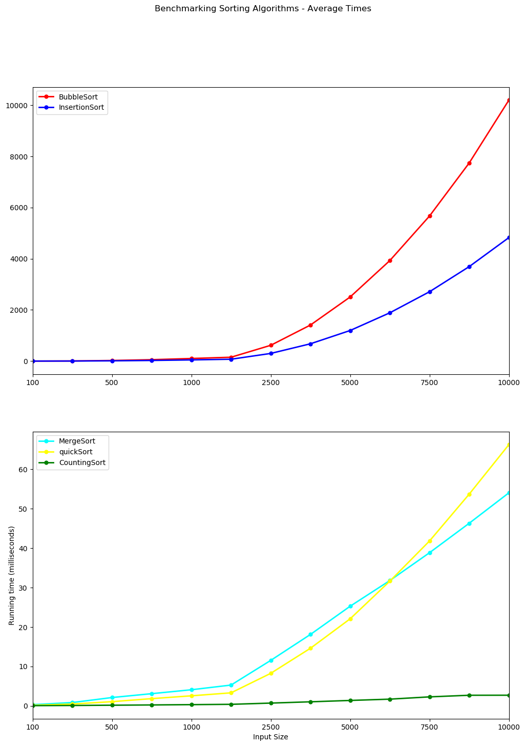
Bubble Sort and Insertion Sort are plotted together below on a single plot while Counting Sort, Merge Sort and Quick Sort are plotted on a separate graph. Note the y-axis are on different scales. The y-axis for Bubble Sort and Insertion sort climbs to 10,000 milliseconds or ten seconds while the scale for the other 3 is less than 70 milliseconds.
The growth rate of the Quick Sort and Merge Sort can now be distinguished from each other and from Counting Sort. They display a linearithmic growth. Counting Sorts running time is linear in the number of items and the difference between the maximum and minimum key values. $O(n+k)$.
 </div>
Conclusion
References
- [1]Computational Thinking with Algorithms Lecture notes by Patrick Mannion GMIT, Do- minic Carr at GMIT.
- [2] Algorithms in a Nutshell by George T. Heineman, Gary Pollice and Stanley Selkow
- [3]Problem Solving with Algorithms and Data Structures using Python. Online book by Brad Miller and David Ranum, Luther College
- [4] Algorithms to live by The Computer Science of Human Decisions](Brian Christian and Tom Griffiths
- [4]geeksforgeeks
- https://en.wikipedia.org/wiki/Bubble_sort
- Learn DS & Algorithms
- W3resources.com
- geeksforgeeks.org
- realpython.org
End